Yebelay Berehan – Introduction to Working with Quarto Documents

What is Quarto?

Quarto is a multi-language, next-generation version of R Markdown from Posit.
It includes new features and capabilities while being able to render most existing Rmd files without modification.
Allows integration with R, Python, Julia, and Observable.
Used for creating dynamic content like reports, presentations, blogs, and books.

Why Use Quarto?

Enhances reproducibility by integrating code and documents.
Enables dynamic updates to figures and tables when code changes
Provides scientific markdown features (equations, citations, cross-references)
Facilitates multi-output publishing (web, PDF, Word, books)

Breakdown of a Quarto Document

A .qmd file consists of:

YAML Header: Metadata (title, author, format, options)
Markdown-formatted text: Narrative content
Code Blocks: Embedded analysis with R
Rendering Process: Converts .qmd into output format (HTML, PDF, etc.)
- render it all together, and you have beautiful, powerful, and useful outputs!

Anatomy of a Quarto Document

The key to our reproducible workflow is using Quarto files in RStudio to dynamically render both code and paper narrative.

So what is anatomy of Quarto file?

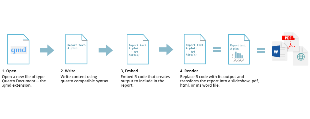
(YAML header, Quarto formatted text, R code chunks”) and how to render them into our final formatted document.

1. YAML header:

What is YAML anyway?

YAML, pronounced “Yeah-mul” stands for “Yet Another Markup Language”.
Quarto default YAML header includes the following metadata surrounded by three dashes ---:

Common key words in YAML

title
author
format
editor

---
title: "Quarto Example"
author: "Yebelay Berehan"
date: today
format: html
editor: visual
execute:
  echo: true
---

In the wizard, you can choose to export your QMD file as a PDF, HTML, or Word document.
These are the default options, but more formats can be added with additional packages.

2. Formatted Text in Quarto

Quarto allows you to format text using Markdown, which enhances plain text beyond a standard R script.
Unlike R scripts, where # starts a comment, plain text in Quarto is simply narrative text. Formatting symbols like ##, **bold**, and < > help structure the document.
Tip: You can also use multiple languages for formatting, including Quarto, HTML, LaTeX, and CSS.

3. Code Blocks in Quarto

Code blocks in Quarto are highlighted in gray and enclosed by triple backticks (```) in source mode.
They start with {} containing options that control how R processes and displays the code.
- These blocks are used for R code, including summary statistics, analysis, tables, and plots.

We can insert these chunk code either clik in the front of render or using short code (ctrl + alt + i) in the source
You can easily copy and paste R scripts into these sections to run them within the document.
You can also use other languages in RStudio, such as R, Python, Bash, and SQL.
There are three main ways to write code in RStudio, each with its own benefits:
- Console : Best for quick calculations and immediate execution, but hard to track and reuse.
- R Script: Allows for organized, reusable code, but less interactive.
- .qmd File: Combines code and text in one document, making it easy to document, modify, and rerun interactively.

The following example shows all the three steps in one

---
title: "Quarto Example"
author: "Yebelay Berehan"
date: today
format: html
---

## MPG

There is a relationship between city and highway mileage.
```{r}
#| label: fig-mpg
library(ggplot2)
ggplot(mpg, aes(x = cty, y = hwy)) + 
  geom_point() + geom_smooth(method = "loess")
```

4. Rendering Your QMD Document

Render it all together, and you have beautiful, powerful, and useful outputs!
Rendering converts your QMD file into a specified format (e.g., PDF, HTML, Word).
Clicking Render compiles the code, checks for errors, and produces the output based on your YAML header settings.

Tip: Enable “Render on Save”to preview changes automatically.

Note that errors in the document may prevent successful rendering.

Tip

In order to create PDFs you will need to install a recent distribution of LaTeX.
We recommend the use of TinyTeX, which you can install with the following command: quarto install tool tinytex.

Formatting Qmd Documents with the sourcein RStudio

List of valid YAML fields

Many YAML fields are common across various outputs
But also each output type has its own set of valid YAML fields and options

---
key: value
---

Output options

---
format: something
---

---
format: html
---

---
format: pdf
---

---
format: revealjs
---

Output option arguments

Indentation matters!

---
format: 
  html:
    toc: true
    code-fold: true
---

YAML validation

Invalid: No space after :

---
format:html
---

Invalid: Read as missing

---
format:
html
---

Valid, but needs next object

---
format: 
  html:
---

YAML validation

There are multiple ways of formatting valid YAML:

Valid: There’s a space after :

format: html

Valid: There are 2 spaces a new line and no trailing :

format:
  html

Valid: format: html with selections made with proper indentation

format: 
  html:
    toc: true

List of valid YAML fields

Many YAML fields are common across various outputs
But also each output type has its own set of valid YAML fields and options
Definitive list: quarto.org/docs/reference/formats/html

Branding & Styling

brand: Define branding (file path, false, or inline object).

format:
  revealjs:
    brand: "branding.yaml"

🔹 Uses branding.yaml for theme customization.

theme: Set a theme (default or custom SCSS).

format:
  revealjs:
    theme: [default, custom.scss]

🔹 Combines the default theme with custom.scss.

anchor-sections: Show an anchor link when hovering over headings.

format:
  revealjs:
    anchor-sections: true

📌 Hover over a title to see a 🔗 link.

tabsets: Enable tabbed content.

::: {.tabset}
### Tab 1
Content for Tab 1.

### Tab 2
Content for Tab 2.
:::

📌 Renders interactive tabs to organize content.

smooth-scroll: Enable smooth scrolling.

format:
  revealjs:
    smooth-scroll: true

📌 Scrolling is animated for a better experience.

Math & Sections

html-math-method: Choose math rendering (mathjax, katex, etc.).
section-divs: Wrap sections in <section> tags.
- Allows precise styling and layout control.

format:
  revealjs:
    html-math-method: mathjax
    section-divs: true

Table of Contents (TOC)

toc: Generate a TOC.
toc-depth: Creates a TOC with up to 2 levels.
toc-location: Position TOC on the left.
- Moves TOC to the left sidebar.

format:
  revealjs:
    toc: true
    toc-depth: 2
    toc-location: left

Numbering & Headings

number-sections: Adds numbered sections
shift-heading-level-by: Shift headings down by 1 level.
number-depth: Customize numbering depth.

syntax in yaml

format:
  revealjs:
    number-sections: true
    shift-heading-level-by: -1
    number-depth: 1

Fonts

mainfont: Set the main font for HTML or LaTeX.
fontsize: Adjust the base font size.
linestretch: Adjust line spacing by 1.5x.

format:
  revealjs:
    mainfont: "Arial"
    fontsize: 14px
    linestretch: 1.5

Colors

fontcolor: Set the text color.
linkcolor: Set the link color.
monobackgroundcolor: Set the background color for code blocks.
backgroundcolor: Set the document background color.

Syntax to set color in yaml

format:
  revealjs:
    fontcolor: "#333333"
    linkcolor: "blue"
    monobackgroundcolor: "#f0f0f0"
    backgroundcolor: "#ffffff"

Layout

cap-location: Place figure and table captions (top, bottom, or margin).

format:
  revealjs:
    cap-location: bottom

📌 Places captions at the bottom of figures and tables.

fig-cap-location: Place figure captions (top, bottom, or margin).

format:
  revealjs:
    fig-cap-location: top

📌 Places figure captions at the top.

tbl-cap-location: Place table captions (top, bottom, or margin).

format:
  revealjs:
    tbl-cap-location: margin

📌 Places table captions in the margin.

Page Layout

classoption: Set LaTeX/PDF class options or KaTeX math alignment.

format:
  revealjs:
    classoption: fleqn

📌 Renders display math equations flush left.

page-layout: Choose page layout (article, full, or custom).

format:
  revealjs:
    page-layout: article

📌 Uses the article layout for the document.

grid: Configure the grid system for HTML pages.

format:
  revealjs:
    grid:
      columns: 12

📌 Sets a 12-column grid layout.

Appendix & Title Block

appendix-style: Choose appendix layout (none, plain, or default).

format:
  revealjs:
    appendix-style: plain

📌 Applies minimal styling to the appendix.

appendix-cite-as: Control citation formats in the appendix.

format:
  revealjs:
    appendix-cite-as: [display, bibtex]

📌 Displays both display and bibtex citation formats.

title-block-style: Choose title block layout (none, plain, or default).

format:
  revealjs:
    title-block-style: default

📌 Uses the default title block styling.

title-block-banner: Add a banner to the title block.

format:
  revealjs:
    title-block-banner: true

📌 Enables a banner with an auto-selected background color.

title-block-banner-color: Set banner text color.

format:
  revealjs:
    title-block-banner-color: "#ffffff"

📌 Sets banner text color to white.

title-block-categories: Enable/disable categories in the title block.

format:
  revealjs:
    title-block-categories: true

📌 Displays categories in the title block.

Margins & Width

max-width: Set a maximum width for the body element.

format:
  revealjs:
    max-width: 800px

📌 Limits the body width to 800px.

margin-left: Set the left margin.

format:
  revealjs:
    margin-left: 2cm

📌 Sets the left margin to 2cm.

margin-right: Set the right margin.

format:
  revealjs:
    margin-right: 2cm

📌 Sets the right margin to 2cm.

margin-top: Set the top margin.

format:
  revealjs:
    margin-top: 2cm

📌 Sets the top margin to 2cm.

margin-bottom: Set the bottom margin.

format:
  revealjs:
    margin-bottom: 2cm

📌 Sets the bottom margin to 2cm.

Code Folding & Summary

code-fold: Collapse code into an HTML <details> tag.

format:
  revealjs:
    code-fold: true

📌 Collapses code blocks, allowing users to expand them on demand.

code-summary: Add summary text for folded code blocks.

format:
  revealjs:
    code-summary: "Click to show code"

📌 Displays “Click to show code” as the summary text.

Code Overflow & Line Numbers

code-overflow: Handle code overflow (scroll or wrap).

format:
  revealjs:
    code-overflow: scroll

📌 Adds a scrollbar for overflowing code.

code-line-numbers: Include line numbers in code blocks.

format:
  revealjs:
    code-line-numbers: true

📌 Adds line numbers to code blocks.

Highlight specific lines:

format:
  revealjs:
    code-line-numbers: "1-3|5-7"

📌 Highlights lines 1-3 first, then 5-7.

Code Copy & Linking

code-copy: Enable a copy icon for code blocks.

format:
  revealjs:
    code-copy: hover

📌 Shows the copy icon when hovering over code blocks.

code-link: Enable hyperlinking of functions to documentation.

format:
  revealjs:
    code-link: true

📌 Links functions in code blocks to their online documentation.

Code Annotations & Tools

code-annotations: Style or hide code annotations.

format:
  revealjs:
    code-annotations: false

📌 Hides code annotations.

code-tools: Add a code tools menu.

format:
  revealjs:
    code-tools: true

📌 Enables a menu for hiding/showing code.

Code Block Styling

code-block-border-left: Add a left border to code blocks.

format:
  revealjs:
    code-block-border-left: "#4CAF50"

📌 Adds a green left border to code blocks.

code-block-bg: Set a background color for code blocks.

format:
  revealjs:
    code-block-bg: "#f0f0f0"

📌 Sets a light gray background for code blocks.

Syntax Highlighting

highlight-style: Set the syntax highlighting style.

format:
  revealjs:
    highlight-style: "pygments"

📌 Uses the Pygments style for syntax highlighting.

syntax-definitions: Use custom KDE syntax definitions.

format:
  revealjs:
    syntax-definitions: "custom.xml"

📌 Applies custom syntax definitions from custom.xml.

indented-code-classes: Specify classes for indented code.

format:
  revealjs:
    indented-code-classes: ["language-python"]

📌 Applies the language-python class to indented code.

Text

The markdown you know from R Markdown will work in Quarto.

Text Formatting

Markdown Syntax	Output
`italics and bold`	italics and bold
`superscript^2^ / subscript~2~`	superscript² / subscript₂
`~~strikethrough~~`	~~strikethrough~~
`verbatim code`	`verbatim code`

Headings

Markdown Syntax	Output
`# Header 1`	Header 1
`## Header 2`	Header 2
`### Header 3`	Header 3
`#### Header 4`	Header 4
`##### Header 5`	Header 5
`###### Header 6`	Header 6

Links

There are several types of “links” or hyperlinks.

Markdown

You can embed [named hyperlinks](https://quarto.org/), 
direct urls like https://quarto.org/, 
and links to [other places](#quarto-anatomy) in  the document.

Output

You can embed named hyperlinks, direct urls like https://quarto.org/, and links to other places in the document.

Lists

Unordered list:

Markdown:

-   unordered list         
    - sub-item 1         
    - sub-item 1         
      -  sub-sub-item 1

Output

unordered list
- sub-item 1
- sub-item 1
  - sub-sub-item 1

Ordered list:

Markdown:

1. ordered list            
2. item 2                  
    i. sub-item 1          
         A.  sub-sub-item 1

Output 1. ordered list
2. item 2 i. sub-item 1 A. sub-sub-item 1

Quotes

Markdown:

> Let us change our traditional attitude to the construction of programs,.... 
> _Donald Knuth, Literate Programming_

. . .

Output:

Let us change our traditional attitude to the construction of programs,…. Donald Knuth, Literate Programming

Divs and spans

Pandoc, and therefore Quarto, can parse “fenced div blocks”:
You can think of a ::: div as a HTML <div> but it can also apply in specific situations to content in PDF:

::: {style="border-left:10px solid red"}
This content can be styled with a border
:::

This content can be styled with a border

[text]{.class} spans can be thought of a <span .class>Text</span> but again are a bit more transferable if using Pandoc/Quarto native attributes.

This is text with [special]{style="color:red;"} formatting.

This is text with special formatting.

Divs with pre-defined classes

These can often apply between formats:

Single class: Two equivalent syntaxes

No {, and no .:

::: unnumbered
Text
:::

{ and .:

::: {.unnumbered}
Text
:::

Multiple classes: use { and ., separate with spaces

::: {.unnumbered .unlisted}
Text
:::

Callouts

::: callout-note
Note that there are five types of callouts, including: 
`note`, `tip`, `warning`, `caution`, and `important`.
:::

Note

Note that there are five types of callouts, including: note, tip, warning, caution, and important.

More callouts

Warning

Callouts provide a simple way to attract attention, for example, to this warning.

Important

Danger, callouts will really improve your writing.

Caution

Here is something under construction.

Caption

Tip with caption.

Footnotes

Pandoc supports numbering and formatting footnotes.

Inline footnotes

Here is an inline note.^[Inlines notes are easier to write, since you don't have to pick an identifier and move down to type the note.]

Here is an inline note.[^1]

Inline footnotes

Here is an footnore reference[^1]

[^1]: This can be easy in some situations when you have a really long note or
  don't want to inline complex outputs.

. . .

Here is an footnote reference[^2]

. . .

Notice in both situations that the footnote is placed at the bottom of the page in presentations, whereas in a document it would be hoverable or at the end of the document.

Code

Anatomy of a code chunk

Code

```{r}
#| label: penguin-stuff
#| message: false
#| output: false
library(tidyverse)
library(palmerpenguins)
penguins |> 
  distinct(species)
```

Has 3x backticks on each end
Engine (r) is indicated between curly braces {r}
Options stated with the #| (hashpipe): #| option1: value

Available code cell options: https://quarto.org/docs/reference/cells/cells-knitr.html

Code, who is it for?

The way you display code is very different for different contexts.
In a teaching scenario like today, I really want to display code.
In a business, you may want to have a data-science facing output which displays the source code AND a stakeholder-facing output which hides the code.

Code

If you simply want code formatting but don’t want to execute the code:

Option 1: Use 3x back ticks + the language ```r

```r
head(penguins)
```

. . .

Option 2: Add eval: false as chunk option

Code

```{r}
#| eval: false
head(penguins)
```

Showing and hiding code with `echo`

The echo option shows the code when set to true and hides it when set to false.
If you want to both execute the code and return the full code including backticks (like in a teaching scenario) echo: fenced is your friend!

Source:

```{{r}}
#| echo: fenced
1 + 1
```

Output:

Code

```{r}
1 + 1
```

[1] 2

Tables and figures

In reproducible reports and manuscripts, the most commonly included code outputs are tables and figures.
So they get their own special sections in our deep dive!

Tables

Markdown tables

Markdown:

| Right | Left | Default | Center |
|------:|:-----|---------|:------:|
|   12  |  12  |    12   |    12  |
|  123  |  123 |   123   |   123  |
|    1  |    1 |     1   |     1  |

Output:

Right	Left	Default	Center
12	12	12	12
123	123	123	123
1	1	1	1

Grid tables

Markdown:

+---------------+---------------+--------------------+
| Fruit         | Price         | Advantages         |
+===============+===============+====================+
| Bananas       | $1.34         | - built-in wrapper |
|               |               | - bright color     |
+---------------+---------------+--------------------+
| Oranges       | $2.10         | - cures scurvy     |
|               |               | - tasty            |
+---------------+---------------+--------------------+

: Sample grid table.

Grid tables

Output:

Sample grid table.
Fruit	Price	Advantages
Bananas	$1.34	built-in wrapper bright color
Oranges	$2.10	cures scurvy tasty

Grid tables: Alignment

Alignments can be specified as with pipe tables, by putting colons at the boundaries of the separator line after the header:

+---------------+---------------+--------------------+
| Right         | Left          | Centered           |
+==============:+:==============+:==================:+
| Bananas       | $1.34         | built-in wrapper   |
+---------------+---------------+--------------------+

For headerless tables, the colons go on the top line instead:

+--------------:+:--------------+:------------------:+
| Right         | Left          | Centered           |
+---------------+---------------+--------------------+

Grid tables: Authoring

Note that grid tables are quite awkward to write with a plain text editor because unlike pipe tables, the column indicators must align.
The Visual Editor can assist in making these tables!

Tables from code

The knitr package can turn data frames into tables with knitr::kable():

Code

library(knitr)
head(penguins) |> 
  kable()

species	island	bill_length_mm	bill_depth_mm	flipper_length_mm	body_mass_g	sex	year
Adelie	Torgersen	39.1	18.7	181	3750	male	2007
Adelie	Torgersen	39.5	17.4	186	3800	female	2007
Adelie	Torgersen	40.3	18.0	195	3250	female	2007
Adelie	Torgersen	NA	NA	NA	NA	NA	2007
Adelie	Torgersen	36.7	19.3	193	3450	female	2007
Adelie	Torgersen	39.3	20.6	190	3650	male	2007

Tables from code

If you want fancier tables, try the gt package and all that it offers!

Code

library(gt)
library(palmerpenguins)
head(penguins) |> 
  gt() |>
  tab_style(
    style = list(
      cell_fill(color = "pink"),
      cell_text(style = "italic")),
    locations = cells_body(
      columns = bill_length_mm,
      rows = bill_length_mm > 40))

species	island	bill_length_mm	bill_depth_mm	flipper_length_mm	body_mass_g	sex	year
Adelie	Torgersen	39.1	18.7	181	3750	male	2007
Adelie	Torgersen	39.5	17.4	186	3800	female	2007
Adelie	Torgersen	40.3	18.0	195	3250	female	2007
Adelie	Torgersen	NA	NA	NA	NA	NA	2007
Adelie	Torgersen	36.7	19.3	193	3450	female	2007
Adelie	Torgersen	39.3	20.6	190	3650	male	2007

Figures

Markdown figures

![Penguins playing with a Quarto ball](images/penguins-quarto-ball.png)

Penguins playing with a Quarto ball

Markdown figures with options

![Penguins playing with a Quarto ball](images/penguins-quarto-ball.png){fig-align="left"}

![](images/penguins-quarto-ball.png){fig-align="right" fig-alt="Illustration of two penguins playing with a Quarto ball."}

Illustration of two penguins playing with a Quarto ball.

Subfigures

Markdown:

::: {#fig-penguins layout-ncol=2}

![Blue penguin](images/blue-penguin.png){#fig-blue width="250px"}

![Orange penguin](images/orange-penguin.png){#fig-orange width="250px"}

Two penguins

:::

Subfigures

Output:

Figure divs

Markdown:

::: {#fig-penguin}

<iframe width="560" height="315" src="https://www.youtube.com/embed/q3uXXh1sHcI"</iframe>

Baby penguin tries to make friends
:::

Figure divs

Output:

Figure 2: Baby penguin tries to make friends

Last paragraph in the div block is used as the figure caption.

Finding the figures to include

In places like markdown, YAML, or the command line/shell/terminal, you’ll need to use absolute or relative file paths:

Absolute = BAD: "/Users/mine/quarto-asa-nebraska" - Whose computer will this work on?

Relative = BETTER:
"../ = up one directory, ../../ = up two directories, etc.
/.. or / = start from root directory of your current computer

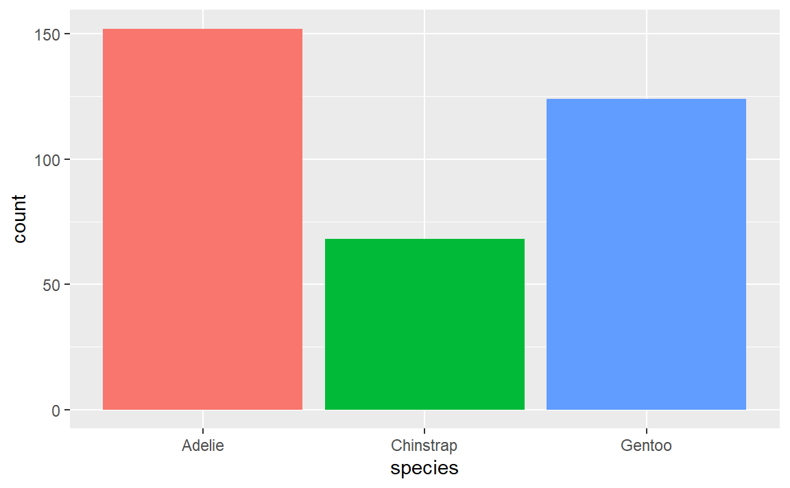
Figures from code

Code

```{r}
#| fig-width: 6
#| fig-asp: 0.618

ggplot(penguins, aes(x = species, fill = species)) +
      geom_bar(show.legend = FALSE)
```

Cross references

Help readers to navigate your document with numbered references and hyperlinks to entities like figures and tables.
Cross referencing steps:
- Add a caption to your figure or table.
- Give an id to your figure or table, starting with fig- or tbl-.
- Refer to it with @fig-... or @tbl-....

Figure cross references

The presence of the caption (Blue penguin) and label (#fig-blue-penguin) make this figure referenceable:

Markdown:

See @fig-blue-penguin for a cute blue penguin.
![Blue penguin](images/blue-penguin.png){#fig-blue-penguin}

Output:

See Figure 3 for a cute blue penguin.

Figure 3: Blue penguin

Table cross references

The presence of the caption (A few penguins) and label (#tbl-penguins) make this table referenceable:

Markdown:

See @tbl-penguins for data on a few penguins.

```{r}
#| label: tbl-penguins
#| tbl-cap: A few penguins

head(penguins) |> 
 gt()
```

Output: See Table 1 for data on a few penguins.

Code

head(penguins) |> 
  gt()

Table 1: A few penguins

species	island	bill_length_mm	bill_depth_mm	flipper_length_mm	body_mass_g	sex	year
Adelie	Torgersen	39.1	18.7	181	3750	male	2007
Adelie	Torgersen	39.5	17.4	186	3800	female	2007
Adelie	Torgersen	40.3	18.0	195	3250	female	2007
Adelie	Torgersen	NA	NA	NA	NA	NA	2007
Adelie	Torgersen	36.7	19.3	193	3450	female	2007
Adelie	Torgersen	39.3	20.6	190	3650	male	2007

Quarto presentations

Components

Metadata: YAML
Text: Markdown
Code: Executed via knitr or jupyter

. . .

Weave it all together, and you have a beautiful, functional slide deck!

Our turn

Let’s build a presentation together from hello-penguins-slides.qmd and showcase the following features of Quarto presentations:

Hierarchy, headers, and document outline
Incremental lists
Columns
Code, output location, code highlighting
Logo and footer
Making things fit on a slide
Chalkboard
Publishing your presentation to Quarto Pub

Quarto presentation formats

revealjs
- essentially the replacement for xaringan, but with Pandoc-native syntax
beamer for LaTeX slides
PowerPoint for when you have to collaborate via MS Office

Formatting Qmd Documents with the Visual Editor in RStudio

The visual editor in RStudio simplifies formatting and enhances productivity when working with Quarto documents.
It provides a user-friendly interface for composing longer articles and data analyses, similar to working with Google Docs or other document editors.

Switching to the Visual Editor

Quarto Markdown (.qmd) documents can be edited in either source mode or visual mode.
To enable the visualmode n the top-left corner of the document toolbar.
Once in visual mode, a formatting toolbar appears, allowing you to:
- Apply styling (bold, italics, headings)
- Insert links and images
- Create tables
- Format content without writing raw Markdown syntax
You can switch between source and visual mode anytime, and your editing location, undo, and redo history will be preserved.

The editor toolbar includes buttons for the most commonly used formatting commands:

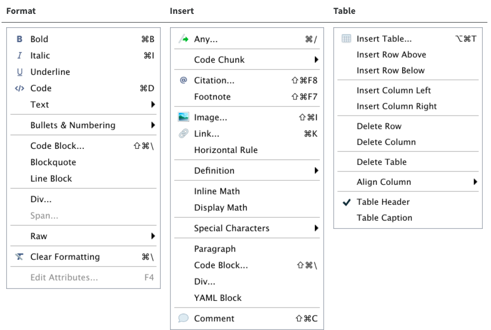
Applying Formatting in the Visual Editor

The visual editor in RStudio allows you to apply formatting effortlessly in Quarto (.qmd) documents.
Below are key formatting tasks and how to perform them efficiently.

Applying Emphasis (Italics & Bold)

At the top of your document, you may have a recommended citation that includes the journal title “Data in Brief.”
To emphasize it in italics:
- Select “Data in Brief” in the text.
  - Click on the italic (“I”) icon in the toolbar.
  - Done! The text now appears in italics.
📌 Tip: If you need bold text, click the “B” icon instead.

Adding Links

To add a hyperlink to a DOI reference in your citation:
- Select the text where you want to insert the link.
- Click the link icon in the toolbar.
- Paste the DOI into the URL field and confirm.
📌 Pro Tip: You can also use the Insert Menu or keyboard shortcuts (hover over the icons to see shortcut hints).
❌ If you mistakenly apply a shortcut, simply press Backspace to undo it.

Adding Headings

Headings help structure your document and improve readability.
- Let’s apply a Level 2 heading to sections like Abstract and Value of the Data:
Select the section title (e.g., “Abstract”).
Click on “Normal” (left side of the toolbar) and choose “Heading 2” from the dropdown.

📌 Tip: Keyboard shortcuts for headings appear next to their names in the menu.

Creating Tables

Manually creating tables in Markdown (.qmd) can be tedious.
However, the visual editor simplifies the process.
To insert a 10-row, 2-column table:
Click on the table icon in the toolbar.
Select the number of rows and columns needed.
Add content to each cell.
Optional: Add a caption (recommended for clarity).
You can also:
- Delete or add rows/columns easily.
- Use a bold header (default but customizable).
- Adjust text alignment inside table cells.

📌 Tip: To clear formatting, select the text and click the crossed “T” icon.

Enhancing Your Quarto Document with Lists, Images, Formulas, and Shortcuts

The visual editor in RStudio simplifies document formatting, making it easy to create lists, insert images, add mathematical formulas, and use shortcuts efficiently.

Creating Bullet and Numbered Lists

Lists help organize information clearly and improve readability.

To create a bullet list:

Select the text.
Click the bullet list icon (•) in the toolbar.

To create a numbered list:

Select the text.
Click the numbered list icon (1,2,3) in the toolbar.

📌 Tip: You can indent (sink) or outdent (lift) items using the increase/decrease indent buttons.

Adding Images

Including static images in your manuscript is simple with the visual editor.

Click the image icon (🖼️) in the toolbar.
Browse and upload the image file.
Add an optional caption and image title.
Adjust image size and alignment if needed.

📌 Example: Insert an image for Figure 1 (Fig. 1).

Adding Formulas

To insert mathematical equations in Quarto, you have three options:

Using the Insert Menu: Click on Insert → Equation.
Using a Keyboard Shortcut: Press ⌘ / (Mac) or Ctrl / (Windows).
Typing in Markdown Format:
- For inline math, type: $E = mc^2$
- For display math (block equation), type:

$$E = mc^2$$

📌 Tip: The font color and style change automatically when a math formula is detected.

Keyboard Shortcuts for Faster Editing

To speed up your workflow, consider these commonly used shortcuts:

pushpin: **Tip:** You can use both **traditional shortcuts** (e.g., ⌘ B for bold) and **Markdown syntax** (e.g., `**bold**` for bold text).
Action	Mac Shortcut	Windows Shortcut
Bold text	⌘ B	Ctrl B
Italic text	⌘ I	Ctrl I
Insert link	⌘ K	Ctrl K
Heading Level 2	## + Space	## + Space
Insert code block	``` + Enter	``` + Enter

Advanced Editing Features in Quarto’s Visual Editor

Beyond basic formatting, Quarto’s visual editor allows for advanced content styling, structured layouts, and enriched documents.
Let’s explore additional formatting options, including HTML elements, blockquotes, footnotes, code chunks, and fenced divs for enhanced styling.

Other Editing Features

Inserting Images:
Browse for an image file or simply copy and paste it into the document.
- Adding Special Elements:
Insert HTML, line blocks, blockquotes, and footnotes for structured content.
Use the Insert menu for easy access. 📌 Up Next: Learn how to add code chunks to your .qmd document.

Bonus: Advanced Styling with Fenced Divs

Quarto allows for custom styling and layout control using fenced divs.
These help in grouping content, adding borders, and creating column layouts
- all while maintaining consistency across different output formats.

Basic Syntax for Fenced Divs

Start and end with at least three colons (:::).
Use curly brackets {} to define a class for styling.

Example 1: Adding a Border Around Text

::: {.border}   
Example of some content with a border.   
:::

✅ Output: A boxed section that highlights important content.

Example 2: Creating Multiple Columns

To separate content into two columns, use the .columns class:

:::: {.columns}   
::: {.column width="50%"}   
Some content in the left column   
:::   
::: {.column width="50%"}   
Some content in the right column   
:::   
::::

✅ Output: Two side-by-side columns for better layout control.

Time to Render!

After applying these edits, render the document to see how it looks in the final output.

Key Takeaways

✅ The visual editor simplifies formatting, requiring minimal Quarto knowledge. ✅ You can structure documents with inline code, dynamic content, and special styling. ✅ Fenced divs allow for customized layouts like borders, columns, and sections.

📌 Next Steps: Explore Quarto’s Divs and Spans documentation for more advanced styling techniques! 🚀

Rendering Code in Quarto Documents

In the previous episode, we explored how to run code chunks and preview their output.
Now, let’s discuss how to render the final document while controlling the appearance of code and outputs.

How Rendering Works in Quarto

The Render button in Quarto follows a two-step process:

Runs all code chunks automatically.
Generates the final document in the chosen output format (e.g., HTML, PDF, Word).

Handling Code Output in the Final Document

You might notice that code messages, warnings, and raw outputs appear in the rendered document, even if you didn’t intend for them to be included.

📌 Example Issue:
When running analysis, messages like warnings, console outputs, or function messages can clutter the final document.

Solution: Use Code Chunk Options to control what appears in the output.

Key Code Chunk Options in Quarto

Code chunk options are written in YAML format within {} after #| inside a Quarto code chunk:

#| option: value

white_check_mark: **Common Code Chunk Options**
Option	Description
`include`	(TRUE/FALSE) Whether to include the output in the document (default: `TRUE`).
`eval`	(TRUE/FALSE) Whether to evaluate the code. Use `eval = c(1,3)` to run only parts of the code.
`echo`	(TRUE/FALSE) Show or hide the code chunk itself.
`results`	(markup/hide/asis/hold/true/false) Controls how the text output is displayed.
`warning`	(TRUE/FALSE) Whether to show warnings in the final document.
`message`	(TRUE/FALSE) Whether to display function messages.

Cleaning Up Your Quarto Output

To improve readability and hide unwanted outputs, add these options inside your code chunk:

#| echo: false #| message: false #| warning: false #| results: false

🔹 What This Does:
✔ No source code in the rendered output (echo: false).
✔ No messages or warnings in the final document (message: false, warning: false).
✔ Only figures and outputs remain (results: false).

Example: Clean Output for a Plot

#| echo: false #| message: false #| warning: false 
library(ggplot2)  
ggplot(mtcars, aes(x = hp, y = mpg)) + geom_point()

✅ Final Output:
A clean figure with no extra text in the HTML/PDF document.

Time to Render!

Click the Render button and check if your document now looks clean and polished.

Key Takeaways

✔ The Render button runs all code chunks and generates the final document.
✔ Code chunk options help control output visibility in the document.
✔ Use echo: false, message: false, and warning: false to remove unnecessary clutter.
✔ Figures and key results will still appear, keeping the document professional and concise.

📌 Next Steps: Explore advanced chunk options, caching, and custom styling in Quarto! 🚀

Rendering Code in Quarto Documents

When working with Quarto, code chunks allow you to test and preview the code output. However, to generate a final output (e.g., HTML, PDF, or Word document), you must render the document.

Rendering Process

Code Execution: All code chunks are executed automatically.
Document Rendering: If there are no errors, the entire Quarto document is compiled into the selected output format.

However, default rendering includes unwanted outputs such as messages, warnings, and other results that may clutter the document. To control this, Quarto provides code chunk options.

Code Chunk Options for Better Output

Quarto has over 50 different code chunk options for controlling evaluation, text output, formatting, caching, and figures. Here are some common ones:

Code Evaluation & Output Control

Option	Description
`include = FALSE`	Runs the code but does not display it or its output.
`eval = FALSE`	Prevents the code from executing.
`echo = FALSE`	Hides the source code but shows the output.
`results = 'hide'`	Hides textual output but still allows plots to be displayed.
`warning = FALSE`	Suppresses warnings from appearing in the document.
`message = FALSE`	Hides messages (e.g., package loading messages).

Example Usage

CopyEdit

#| echo: false #| message: false #| warning: false

This setup ensures:

The source code is hidden in the final output.
Messages and warnings are only printed to the console (not included in the document).

Customizing Figures in Quarto

Quarto provides several options for controlling figure appearance, including width, height, alignment, and captions.

Option	Description
`fig-width` & `fig-height`	Sets figure dimensions (in inches).
`out-width` & `out-height`	Controls the output size in the document (scaling possible).
`fig-align`	Aligns figures (`'left'`, `'right'`, `'center'`).
`fig-cap`	Adds a caption to the figure.
`fig-link`	Adds a hyperlink to the figure.
`fig-alt`	Specifies alternative text for accessibility.

Example Usage

CopyEdit

#| fig-width: 6 #| fig-height: 4 #| fig-align: "center" #| fig-cap: "This is a sample figure." ggplot(df, aes(x = x_variable, y = y_variable)) + geom_point()

The figure width is 6 inches, and the height is 4 inches.
The figure is center-aligned in the document.
A caption is added.

Best Practices for Loading Data and Packages

To improve document organization and rendering speed:
✅ Load all necessary libraries and datasets at the beginning of the document.
✅ Avoid reloading data and packages in multiple code chunks.

Example

Code

# Load libraries 
library(tidyverse) 
library(BayesFactor) 
library(patchwork)  # Load data 
df <- read_csv("../data/processed/preprocessed-GARP-TSST-data.csv")`

Why is this important?

Libraries and datasets loaded in the first chunk remain available throughout the document.
This prevents unnecessary repetition and saves rendering time.
It also makes it easier to track dependencies.

Order Matters!

🚨 If you load data before loading the necessary libraries, you may get errors.
💡 Solution: Load all required packages before loading your dataset.

Using Inline Code for Dynamic Text

Sometimes, instead of a full code chunk, you only need a quick calculation inside your narrative.
Quarto supports inline code, which allows dynamic values inside text.

Inline Code Syntax

Use backticks with r to embed R code inside text:

`` The dataset contains  observations. ``

Quarto replaces the inline code with the actual result during rendering.