Yebelay Berehan – Advanced Data Managment

Data Manipulation and Claning using `dplyr()` package

What is Tidyverse?

The tidyverse is a collection of R packages designed for data science.
- All packages share an underlying design philosophy, grammar, and data structures.
All packages included in tidyverse are automatically installed when installing the tidyverse package:

Code

library("tidyverse"); tidyverse_packages()

Then to work functions under tidyverse package we must always load the package into the workplace.

Code

library(tidyverse)

Some packages under tidyverse are considered core packages and others called friend packages.

install.packages(“tidyverse”)

Core tidyverse

tibble, for tibbles, a modern re-imagining of data frames
readr, for data import
tidyr, for data tidying
ggplot2, for data visualization
dplyr, for data manipulation
stringr, for strings
forcats, for factors
purrr, for functional programming

Friends for data import or export (beyond readr)

readxl, for xls and xlsx files
haven, for SPSS, SAS, and Stata files
jsonlite, for JSON
xml2, for XML
httr, for web APIs
rvest, for web scraping
DBI, for databases

Friends for date wrangling

lubridate and hms, for date/times

Friends for modeling

modelr and broom for model/tidy data

For this training we manly use the following Core Packages

Intro to `dplyr` package

dplyr is part of tidyverse provides a grammar (the verbs) for data manipulation.

The key operator and the essential verbs are:

Function	Description	Operates on
`filter()`	pick rows matching criteria	rows
`slice()`	pick rows using indices	rows
`arrange()`	reorder rows	rows
`select()`	pick columns by name	columns
`mutate()`	add new variables	columns
`summarise()`	reduce variables to values	groups of rows
`relocate()`	to change column positions	columns

… many more.

%>% or |> : the “pipe” operator used to connect multiple verb actions together into a pipeline.

Tools → Global Options → Code → Editing → Use Native Pipe Operator (|>)

Select Columns from a Dataset `select()`:

select(): To extract variables

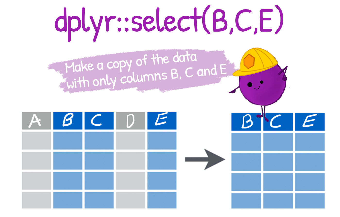
select() columns
select columns (variables)
no quotes needed around variable names
can be used to rearrange columns
uses special syntax that is flexible and has many options

Note that the column names are not quoted; you access the column name as if you are calling the name of an object or variable

Ways to Use `select()` in dplyr

Method	Description	Example
using column name	Select specific columns by their names.	`select(col1, col2)`
By position	Select columns by their positions.	`select(1, 3)`
Using a range	Use `:` to select columns	`select(col1:col5); select(2:4)`
Exclude columns	Use `-` to exclude specific columns	select(-col3); select(-(2:4));``select(!starts_with("A"))
Use pattern	Use helper functions based on patterns.	`select(starts_with("prefix"))` `select(ends_with("suffix"))` `select(contains("text"))`
Select by type	Use `where()` to select based on type or condition.	`select(where(is.numeric))` `select(where(~ n_distinct(.) > 5))`
Select columns using `matches()`	Use a regular expression to select columns matching a specific pattern.	select(matches("col[1-3]")); ``select(matches("^var\\d+"))
Select all columns except some	Use `everything()` to re-order or select all columns except specific ones.	`select(col1, everything())` `select(-starts_with("temp"))`
Rearrange columns	Move specific columns to the front while retaining all others.	`select(col1, col3, everything())`

About the data

Data from the CDC’s Youth Risk Behavior Surveillance System (YRBSS)

complex survey data
national school-based survey conducted by CDC
monitors six categories of health-related behaviors
- that contribute to the leading causes of death and disability among youth and adults
- including alcohol & drug use, unhealthy & dangerous behaviors, sexuality, and physical activity
the data in yrbss_demo.csv are a subset of data in the R package yrbss

Code

library(readr)
yrb_data <- read_csv("data/yrbss.csv")

We can have a look at the data and its structure by using the glimpse() function from the dplyr package.

Pipe perator (`|>`)

Pipes in R look like |> and strings together commands to be performed sequentially
The pipe passes the data frame output that results from the function right before the pipe to input it as the first argument of the function right after the pipe.

Code

third(second(first(x)))

This nesting is not a natural way to think about a sequence of operations.
The |> operator allows you to string operations in a left-to-right fashion.

Code

first(x) |>
second |> third

Advantages of Pipe oprator

Pipes used to reduce multiple steps, that can be hard to keep track of.
less redundant code
Easy to read and write because functions are executed in order
- Difficult to read if too many functions are nested
Look at the three syntax

Code

data1<-filter(sampledata, Age > 15) #<<
data2<-select(data1, Sex, Weight1, Age) #<<

Code

non_piped <-select(filter(mydata, Age>15), Sex, Weight1, Age) #<<

Code

pipeddata<-mydata |> filter(Age > 15) |> select(Sex, Weight1, Height1, Age)#<<

select a column by name: `select(col1, col2, col3, ...)`

Code

library(dplyr)
yrb_data1 <- yrb_data |> 
  select(age, sex, grade)
yrb_data1

# A tibble: 20,000 × 3
   age                   sex    grade
   <chr>                 <chr>  <chr>
 1 15 years old          Female 10th 
 2 17 years old          Female 12th 
 3 18 years old or older Male   11th 
 4 15 years old          Male   10th 
 5 14 years old          Male   9th  
 6 17 years old          Male   9th  
 7 16 years old          Male   11th 
 8 17 years old          Male   12th 
 9 18 years old or older Male   12th 
10 14 years old          Male   10th 
# ℹ 19,990 more rows

Selecting column ranges with `:`

The : operator selects a range of consecutive variables:

Code

yrb_data |>  select(age:race4) |>  head(3)

# A tibble: 3 × 4
  age                   sex    grade race4          
  <chr>                 <chr>  <chr> <chr>          
1 15 years old          Female 10th  White          
2 17 years old          Female 12th  White          
3 18 years old or older Male   11th  Hispanic/Latino

We can also specify a range with column numbers:

Code

yrb_data |> select(1:4) |> head(3)

# A tibble: 3 × 4
  record age                   sex    grade
   <dbl> <chr>                 <chr>  <chr>
1 931897 15 years old          Female 10th 
2 333862 17 years old          Female 12th 
3  36253 18 years old or older Male   11th

Excluding columns with `!` or `-`

The exclamation point negates a selection:

Code

yrb_data |> select(!record) |> head(2)

# A tibble: 2 × 7
  age          sex    grade race4 race7   bmi stweight
  <chr>        <chr>  <chr> <chr> <chr> <dbl>    <dbl>
1 15 years old Female 10th  White White  17.2     54.4
2 17 years old Female 12th  White White  20.2     57.2

To drop a range of consecutive columns, we use, for example,!age:grade:

Code

yrb_data |> select(!age:grade) |> head(2)

# A tibble: 2 × 5
  record race4 race7   bmi stweight
   <dbl> <chr> <chr> <dbl>    <dbl>
1 931897 White White  17.2     54.4
2 333862 White White  20.2     57.2

To drop several non-consecutive columns, place them inside !c():

Code

yrb_data |> select(!c(race4, race7)) |> head(3)

Helper functions: `starts_with()`, `ends_with()` and `contains()`

These two helpers work exactly as their names suggest!

`starts_with()`

Code

yrb_data |> select(starts_with("r")) |> head(2)

# A tibble: 2 × 3
  record race4 race7
   <dbl> <chr> <chr>
1 931897 White White
2 333862 White White

`ends_with()`

Code

yrb_data |> select(ends_with("e")) |> head(3)

# A tibble: 3 × 2
  age                   grade
  <chr>                 <chr>
1 15 years old          10th 
2 17 years old          12th 
3 18 years old or older 11th

`contains()`

contains() helps select columns that contain a certain string:

Code

yrb_data |> select(sex, contains("r")) |> head()

# A tibble: 6 × 5
  sex     record grade race4                     race7                    
  <chr>    <dbl> <chr> <chr>                     <chr>                    
1 Female  931897 10th  White                     White                    
2 Female  333862 12th  White                     White                    
3 Male     36253 11th  Hispanic/Latino           Hispanic/Latino          
4 Male   1095530 10th  Black or African American Black or African American
5 Male   1303997 9th   All other races           Multiple - Non-Hispanic  
6 Male    261619 9th   All other races           <NA>

Another helper function, `everything()`

matches all variables that have not yet been selected.

Code

## First, `bmi`, then every other column.
yrb_data |> select(bmi, everything()) |> head(3)

# A tibble: 3 × 8
    bmi record age                   sex    grade race4           race7 stweight
  <dbl>  <dbl> <chr>                 <chr>  <chr> <chr>           <chr>    <dbl>
1  17.2 931897 15 years old          Female 10th  White           White     54.4
2  20.2 333862 17 years old          Female 12th  White           White     57.2
3  NA    36253 18 years old or older Male   11th  Hispanic/Latino Hisp…     NA

It is often useful for establishing the order of columns.

But this would be painful for larger data frames, data frame. In such a case, we can use everything().

This helper can be combined with many others.

Code

## Bring columns that end with "r" to the front of the data frame
yrb_data |> select(starts_with("r"), everything()) %>% head(3)

# A tibble: 3 × 8
  record race4           race7           age          sex   grade   bmi stweight
   <dbl> <chr>           <chr>           <chr>        <chr> <chr> <dbl>    <dbl>
1 931897 White           White           15 years old Fema… 10th   17.2     54.4
2 333862 White           White           17 years old Fema… 12th   20.2     57.2
3  36253 Hispanic/Latino Hispanic/Latino 18 years ol… Male  11th   NA       NA

You can also select columns based on their data type using select_if().
The common data types to be called are: is.character, is.double, is.factor, is.integer, is.logical, is.numeric.

Code

yrb_data |>  select_if(is.numeric) |>
  glimpse()  # numeric data types only selected (here: integer or double)

Rows: 20,000
Columns: 3
$ record   <dbl> 931897, 333862, 36253, 1095530, 1303997, 261619, 926649, 1309…
$ bmi      <dbl> 17.1790, 20.2487, NA, 27.9935, 24.4922, NA, 20.5435, 19.2555,…
$ stweight <dbl> 54.43, 57.15, NA, 85.73, 66.68, NA, 70.31, 58.97, 123.38, NA,…

Summary for Select() function

There are five ways to select variables in select(data, ...):

By position: yrb_data |> select(1, 2, 4) oryrb_data |> select(1:2).
By name: yrb_data |> select(age, sex), or yrb_data |> select(age:race4).
By function of name: yrb_data |> select(starts_with("r")), or yrb_data |> select(ends_with("e")).
By type: yrb_data |> select(where(is.numeric)),or yrb_data |> select(where(is.character)).
By any combination of the above using the Boolean operators !, &, and |:
- yrb_data |> select(!where(is.numeric)): selects all non-factor variables.
- yrb_data |> select(where(is.numeric) & contains("i")): selects all numeric variables that contains ‘i’.

Also the following are other important function
- _all() if you want to apply the function to all columns
- _at() if you want to apply the function to specific columns (specify them with vars())
- _if() if you want to apply the function to columns of a certain characteristic (e.g. data type)
- _with() if you want to apply the function to columns and include another function within it

Code

yrb_data2 <- yrb_data |> select_all(tolower) |>  glimpse()

Rows: 20,000
Columns: 8
$ record   <dbl> 931897, 333862, 36253, 1095530, 1303997, 261619, 926649, 1309…
$ age      <chr> "15 years old", "17 years old", "18 years old or older", "15 …
$ sex      <chr> "Female", "Female", "Male", "Male", "Male", "Male", "Male", "…
$ grade    <chr> "10th", "12th", "11th", "10th", "9th", "9th", "11th", "12th",…
$ race4    <chr> "White", "White", "Hispanic/Latino", "Black or African Americ…
$ race7    <chr> "White", "White", "Hispanic/Latino", "Black or African Americ…
$ bmi      <dbl> 17.1790, 20.2487, NA, 27.9935, 24.4922, NA, 20.5435, 19.2555,…
$ stweight <dbl> 54.43, 57.15, NA, 85.73, 66.68, NA, 70.31, 58.97, 123.38, NA,…

If we wanted only some of them renamed and kept, we could have used select_at() which specifies columns with vars().

Code

# Select and rename a couple of columns only
yrb_data |>  select_at(vars(sex, age, bmi), toupper) |>  glimpse()

Rows: 20,000
Columns: 3
$ SEX <chr> "Female", "Female", "Male", "Male", "Male", "Male", "Male", "Male"…
$ AGE <chr> "15 years old", "17 years old", "18 years old or older", "15 years…
$ BMI <dbl> 17.1790, 20.2487, NA, 27.9935, 24.4922, NA, 20.5435, 19.2555, 33.1…

Filter cases from the dataset `filter()`

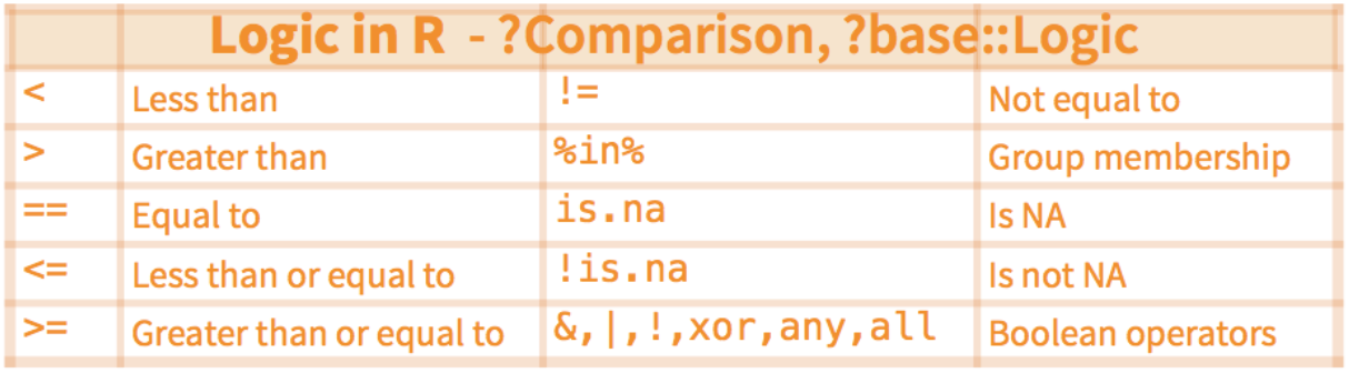
`filter()`: To extract cases

The function filter() is used to filter the dataset to return a subset of all rows that meet one or more specific conditions.

filter(dataframe, logical statement 1, logical statement 2, ...)

Ways to Use `filter()` in dplyr

Method	Description	Example
By specific value	Filter rows where a column equals a specific value.	`filter(col1 == "value")` `filter(col1 != "value")`
By inequality	Filter rows based on inequality conditions.	`filter(col1 > 10)`
Using multiple conditions	Filter rows that satisfy multiple conditions.	`filter(col1 > 10, col2 == "A")`
With logical operators	Using AND (`&) and using OR (`\|)
By range	Filter rows within a range of values using `between()`.	`filter(between(col1, 10, 20))`
By missing values	Filter rows with or without missing values.	`filter(is.na(col1))` `filter(!is.na(col1))`
By string pattern	Filter rows using string functions like `grepl()`.	`filter(grepl("pattern", col1))`
Using `case_when()`	Apply conditional logic for complex filtering.	`filter(case_when(col1 > 10 ~ TRUE, TRUE ~ FALSE))`

Filtering based on exact character variable matches

Note the use of the double equal sign == rather than the single equal sign =.

Code

yrb_data |> select(sex, grade ) |>  filter(grade=="9th")|>  head(3)

# A tibble: 3 × 2
  sex   grade
  <chr> <chr>
1 Male  9th  
2 Male  9th  
3 Male  9th

Code

yrb_data |> select(sex, grade)|> filter(sex == "Male") |> head(3)

# A tibble: 3 × 2
  sex   grade
  <chr> <chr>
1 Male  11th 
2 Male  10th 
3 Male  9th

Similarly you can use the other operators:
- filter(grade != "9th") will select everything except the grade 9 rows.

If you want to select more than one category value you can use the %in% operator.

Code

yrb_data |> 
  select(sex, age, grade ) |> 
  filter(grade %in% c("9th", "11th")) |> head(3)

The %in% operator used to deselect certain groups as well, using !%in%.

Code

yrb_data |> select(sex, age, race4) |> 
  filter(!grade %in% c("Hispanic/Latino", "white")) |> 
  head(3)

To select all individuals with a bmi between 22 and 30, use:

Code

yrb_data |> 
  select(sex, age, bmi) |> 
  filter(between(bmi, 22, 30))

Code

yrb_data |> 
  select(sex, age, bmi) |> 
  filter(bmi >= 22, bmi <= 30)

Filtering based on multiple conditions

The filter option also allows AND and OR style filters:
filter(condition1, condition2) will return rows where both conditions are met.
filter(condition1, !condition2) will return all rows where condition one is true but condition 2 is not.
filter(condition1 | condition2) will return rows where condition 1 and/or condition 2 is met.
filter(xor(condition1, condition2) will return all rows where only one of the conditions is met, and not when both conditions are met.

Code

yrb_data |> select(sex, age, bmi, stweight, grade) |> 
  filter(bmi > 20, (stweight > 50 | grade != "12th")) |> 
  head(3)

# A tibble: 3 × 5
  sex    age            bmi stweight grade
  <chr>  <chr>        <dbl>    <dbl> <chr>
1 Female 17 years old  20.2     57.2 12th 
2 Male   15 years old  28.0     85.7 10th 
3 Male   14 years old  24.5     66.7 9th

Example with `xor()`

Code

yrb_data |> 
  select(bmi, stweight) |> 
  filter(xor( bmi > 20, 
    stweight > 50)) |> 
  head(4)

# A tibble: 4 × 2
    bmi stweight
  <dbl>    <dbl>
1  17.2     54.4
2  19.3     59.0
3  21.6     49.9
4  19.3     54.4

To filter out empty rows, use !is.na().

Code

yrb_data |>  
  select(bmi, stweight) |> 
  filter(!is.na(bmi)) |> 
  head(4)

# A tibble: 4 × 2
    bmi stweight
  <dbl>    <dbl>
1  17.2     54.4
2  20.2     57.2
3  28.0     85.7
4  24.5     66.7

Filtering across multiple columns

Method	Description	Example
`across()`	Filter rows based on conditions across multiple columns.	`filter(across(starts_with("col"), ~ .x > 10))`
`filter_at()`	Filter rows based on selected columns using conditions.	`filter_at(vars(col1, col2), all_vars(. > 10))`
`filter_if()`	Filter rows based on a condition for specific column types.	`filter_if(is.numeric, all_vars(. > 10))`
`filter_all()`	Apply the same condition across all columns.	`filter_all(all_vars(. > 0))`
`across()` and `any_vars()`	Keep rows where any column satisfies a condition.	`filter(across(starts_with("col"), any_vars(. > 10)))`
`across()` and `all_vars()`	Keep rows where all selected columns satisfy a condition.	`filter(across(ends_with("score"), all_vars(. >= 50)))`
`between()` in multiple columns	Filter rows where values fall within a range.	`filter(across(c(col1, col2), ~ between(.x, 10, 20)))`

across() is the modern and flexible replacement for filter_at(), filter_if(), and filter_all().
all_vars() ensures all selected columns satisfy the condition.
any_vars() ensures at least one selected column satisfies the condition.

`filter_all()`

Used to wrap the condition in any_vars().
- For example to find the string “symp” across all columns,

Code

library(stringr)
yrb_data |> 
   filter_all(any_vars(str_detect(., pattern = "Black"))) |> head()

The same can be done for numerical values: This code will retain any rows that has any value above 120:

Code

yrb_data |>  
  select(bmi, stweight) |> 
  filter_all(any_vars(. > 120)) |> head(4)

# A tibble: 4 × 2
    bmi stweight
  <dbl>    <dbl>
1  33.1     123.
2  38.2     150.
3  40.4     128.
4  38.3     131.

any_vars() statement is equivalent to OR, and
all_vars()is an equivalent for AND.

The below code will retain any rows where all values are below 15.

Code

yrb_data |>  
  select(bmi, stweight) |> 
  filter_all(any_vars(. < 15)) |> head()

# A tibble: 6 × 2
    bmi stweight
  <dbl>    <dbl>
1  13.2     47.6
2  15.0     40.8
3  13.9     59.0
4  13.2     27.7
5  15.0     NA  
6  15.0     55.8

`filter_if()`

to find out all data rows where we NA in the first few columns use filter_all(any_vars(is.na(.)))
Using filter_if() I can filter on character variables.

Code

yrb_data |> 
   filter_if(is.numeric, any_vars(is.na(.))) |> head()

# A tibble: 6 × 8
  record age                   sex   grade race4            race7   bmi stweight
   <dbl> <chr>                 <chr> <chr> <chr>            <chr> <dbl>    <dbl>
1  36253 18 years old or older Male  11th  Hispanic/Latino  Hisp…    NA       NA
2 261619 17 years old          Male  9th   All other races  <NA>     NA       NA
3 180494 14 years old          Male  10th  Black or Africa… Blac…    NA       NA
4  31226 15 years old          Male  10th  All other races  <NA>     NA       NA
5 109404 16 years old          Male  11th  White            White    NA       NA
6 180968 15 years old          Male  9th   White            White    NA       NA

Or

Code

yrb_data |> 
   filter_if(is.character, all_vars(!is.na(.))) |> head()

# A tibble: 6 × 8
   record age                   sex    grade race4          race7   bmi stweight
    <dbl> <chr>                 <chr>  <chr> <chr>          <chr> <dbl>    <dbl>
1  931897 15 years old          Female 10th  White          White  17.2     54.4
2  333862 17 years old          Female 12th  White          White  20.2     57.2
3   36253 18 years old or older Male   11th  Hispanic/Lati… Hisp…  NA       NA  
4 1095530 15 years old          Male   10th  Black or Afri… Blac…  28.0     85.7
5 1303997 14 years old          Male   9th   All other rac… Mult…  24.5     66.7
6  926649 16 years old          Male   11th  All other rac… Asian  20.5     70.3

`filter_at()`

select columns to which the change should happen via the vars() argument.
Use all_vars() if all columns need to return TRUE, or any_vars() in case just one variable needs to return TRUE.

Code

yrb_data |> 
   filter_at(vars(bmi, stweight), all_vars(.> 50))|> head(3)

# A tibble: 3 × 8
   record age          sex    grade race4                   race7   bmi stweight
    <dbl> <chr>        <chr>  <chr> <chr>                   <chr> <dbl>    <dbl>
1 1099468 17 years old Male   9th   Black or African Ameri… Blac…  52.0     174.
2  770391 16 years old Female 11th  All other races         Mult…  52.4     161.
3  501097 15 years old Male   12th  All other races         Mult…  50.3     116.

Code

yrb_data |> filter_at(vars(contains("i")), all_vars(.> 50))|> head(3)

Code

yrb_data |> filter_at(vars(contains("i")), any_vars(.< 30))

Adding or Modifying columns using `mutate()`

The dplyr library has the following functions that can be used to add additional variables to a data frame.
mutate() – adds new variables while retaining old variables to a data frame.
transmute() – adds new variables and removes old ones from a data frame.
mutate_all() – changes every variable in a data frame simultaneously.
mutate_at() – changes certain variables by name.
mutate_if() – alterations all variables that satisfy a specific criterion
The mutate() basic syntax is as follows.

Code

data <- mutate(new_variable = existing_variable/3)

data: the fresh data frame where the fresh variables will be placed
new_variable: the name of the new variable
existing_variable: the current data frame variable that you want to modify in order to generate a new variable

Set the new column called height_m

Code

yrb_new <- yrb_data %>% 
  mutate(height_m = sqrt(stweight / bmi))   # use = (not <- or ==) to define new variable

yrb_new %>% select(record, bmi, stweight)

# A tibble: 20,000 × 3
    record   bmi stweight
     <dbl> <dbl>    <dbl>
 1  931897  17.2     54.4
 2  333862  20.2     57.2
 3   36253  NA       NA  
 4 1095530  28.0     85.7
 5 1303997  24.5     66.7
 6  261619  NA       NA  
 7  926649  20.5     70.3
 8 1309082  19.3     59.0
 9  506337  33.1    123. 
10  180494  NA       NA  
# ℹ 19,990 more rows

`transmute()`

A data frame’s variables are added and removed via the transmute() method.
The code that follows demonstrates how to eliminate all of the existing variables and add two new variables to a dataset.

Code

yrb_data |> transmute(root_stweight = sqrt(stweight), 
                   root_bmi = sqrt(bmi))

# A tibble: 20,000 × 2
   root_stweight root_bmi
           <dbl>    <dbl>
 1          7.38     4.14
 2          7.56     4.50
 3         NA       NA   
 4          9.26     5.29
 5          8.17     4.95
 6         NA       NA   
 7          8.39     4.53
 8          7.68     4.39
 9         11.1      5.76
10         NA       NA   
# ℹ 19,990 more rows

`mutate_all()`

The mutate_all() function changes every variable in a data frame at once, enabling you to use the funs() function to apply a certain function to every variable.
The use of mutate_all() to divide each column in a data frame by ten is demonstrated in the code below.
divide 10 from each of the data frame’s variables.

Code

yrb_new1 <- yrb_new %>% select_if(is.numeric)
yrb_new1 |> mutate_all(funs(./10))

# A tibble: 20,000 × 4
    record   bmi stweight height_m
     <dbl> <dbl>    <dbl>    <dbl>
 1  93190.  1.72     5.44    0.178
 2  33386.  2.02     5.72    0.168
 3   3625. NA       NA      NA    
 4 109553   2.80     8.57    0.175
 5 130400.  2.45     6.67    0.165
 6  26162. NA       NA      NA    
 7  92665.  2.05     7.03    0.185
 8 130908.  1.93     5.90    0.175
 9  50634.  3.31    12.3     0.193
10  18049. NA       NA      NA    
# ℹ 19,990 more rows

Remember that you can add more variables to the data frame by supplying a new name to be prefixed to the existing variable name.

Code

yrb_new1 |> mutate_all(funs(mod = ./10)) %>% select(ends_with("mod"))

# A tibble: 20,000 × 4
   record_mod bmi_mod stweight_mod height_m_mod
        <dbl>   <dbl>        <dbl>        <dbl>
 1     93190.    1.72         5.44        0.178
 2     33386.    2.02         5.72        0.168
 3      3625.   NA           NA          NA    
 4    109553     2.80         8.57        0.175
 5    130400.    2.45         6.67        0.165
 6     26162.   NA           NA          NA    
 7     92665.    2.05         7.03        0.185
 8    130908.    1.93         5.90        0.175
 9     50634.    3.31        12.3         0.193
10     18049.   NA           NA          NA    
# ℹ 19,990 more rows

`mutate_at()`

Using names, the mutate at() function changes particular variables.
The use of mutate_at() to divide two particular variables by 10 is demonstrated in the code below:

Code

yrb_new1 |> mutate_at(c("height_m", "stweight"), funs(mod = ./10))

# A tibble: 20,000 × 6
    record   bmi stweight height_m height_m_mod stweight_mod
     <dbl> <dbl>    <dbl>    <dbl>        <dbl>        <dbl>
 1  931897  17.2     54.4     1.78        0.178         5.44
 2  333862  20.2     57.2     1.68        0.168         5.72
 3   36253  NA       NA      NA          NA            NA   
 4 1095530  28.0     85.7     1.75        0.175         8.57
 5 1303997  24.5     66.7     1.65        0.165         6.67
 6  261619  NA       NA      NA          NA            NA   
 7  926649  20.5     70.3     1.85        0.185         7.03
 8 1309082  19.3     59.0     1.75        0.175         5.90
 9  506337  33.1    123.      1.93        0.193        12.3 
10  180494  NA       NA      NA          NA            NA   
# ℹ 19,990 more rows

`mutate_if()`

All variables that match a specific condition are modified by the mutate_if() function.
The mutate_if() function can be used to change any variables of type factor to type character, as shown in the code below.
every character variable can be converted to a factor variable.

Code

yrb_new2 <- yrb_new |> mutate_if(is.character, as.factor)
sapply(yrb_new2, class)

   record       age       sex     grade     race4     race7       bmi  stweight 
"numeric"  "factor"  "factor"  "factor"  "factor"  "factor" "numeric" "numeric" 
 height_m 
"numeric"

The mutate_if() method can be used to round any numeric variables to the nearest whole number using the following example code.
any numeric variables should be rounded to the nearest decimal place.

Code

yrb_new |> mutate_if(is.numeric, round, digits = 1) %>% 
  select(age, bmi, stweight, height_m)

# A tibble: 20,000 × 4
   age                     bmi stweight height_m
   <chr>                 <dbl>    <dbl>    <dbl>
 1 15 years old           17.2     54.4      1.8
 2 17 years old           20.2     57.1      1.7
 3 18 years old or older  NA       NA       NA  
 4 15 years old           28       85.7      1.7
 5 14 years old           24.5     66.7      1.6
 6 17 years old           NA       NA       NA  
 7 16 years old           20.5     70.3      1.8
 8 17 years old           19.3     59        1.8
 9 18 years old or older  33.1    123.       1.9
10 14 years old           NA       NA       NA  
# ℹ 19,990 more rows

Use `across()` inside `mutate()` function

Code

yrb_new |> as_tibble() |> 
  mutate(across(c(bmi, stweight), round)) |> head(4) #<<

# A tibble: 4 × 9
   record age                   sex    grade race4 race7   bmi stweight height_m
    <dbl> <chr>                 <chr>  <chr> <chr> <chr> <dbl>    <dbl>    <dbl>
1  931897 15 years old          Female 10th  White White    17       54     1.78
2  333862 17 years old          Female 12th  White White    20       57     1.68
3   36253 18 years old or older Male   11th  Hisp… Hisp…    NA       NA    NA   
4 1095530 15 years old          Male   10th  Blac… Blac…    28       86     1.75

Code

yrb_new |> as_tibble() |>  
  mutate(across(c(7, 8), round)) |> head(4)#<<

# A tibble: 4 × 9
   record age                   sex    grade race4 race7   bmi stweight height_m
    <dbl> <chr>                 <chr>  <chr> <chr> <chr> <dbl>    <dbl>    <dbl>
1  931897 15 years old          Female 10th  White White    17       54     1.78
2  333862 17 years old          Female 12th  White White    20       57     1.68
3   36253 18 years old or older Male   11th  Hisp… Hisp…    NA       NA    NA   
4 1095530 15 years old          Male   10th  Blac… Blac…    28       86     1.75

Use `across()` inside `mutate()` function

Code

yrb_new |>  as_tibble() |> 
  mutate(across(7:height_m, round)) |> head(4) #<<

# A tibble: 4 × 9
   record age                   sex    grade race4 race7   bmi stweight height_m
    <dbl> <chr>                 <chr>  <chr> <chr> <chr> <dbl>    <dbl>    <dbl>
1  931897 15 years old          Female 10th  White White    17       54        2
2  333862 17 years old          Female 12th  White White    20       57        2
3   36253 18 years old or older Male   11th  Hisp… Hisp…    NA       NA       NA
4 1095530 15 years old          Male   10th  Blac… Blac…    28       86        2

Code

yrb_new |>   as_tibble() |> 
  mutate(across(where(is.double) & !c(record), round)) |> head(4) #<<

# A tibble: 4 × 9
   record age                   sex    grade race4 race7   bmi stweight height_m
    <dbl> <chr>                 <chr>  <chr> <chr> <chr> <dbl>    <dbl>    <dbl>
1  931897 15 years old          Female 10th  White White    17       54        2
2  333862 17 years old          Female 12th  White White    20       57        2
3   36253 18 years old or older Male   11th  Hisp… Hisp…    NA       NA       NA
4 1095530 15 years old          Male   10th  Blac… Blac…    28       86        2

Sort rows with `arrange`

Re-order rows by a particular column, by default in ascending order

Use desc() for descending order.

arrange(data, variable1, desc(variable2), ...)

Example: 1. Let us use the following code to create a scrambled version of the airquality dataset

Code

air_mess <- sample_frac(airquality, 1)
head(air_mess)

  Ozone Solar.R Wind Temp Month Day
1    NA     259 10.9   93     6  11
2    14     334 11.5   64     5  16
3    73     215  8.0   86     8  26
4    34     307 12.0   66     5  17
5    22      71 10.3   77     8  16
6    NA      66 16.6   57     5  25

Sort rows with `arrange()`

Example: 2. Now let us arrange the data frame back into chronological order, sorting by Month then Day

Code

air_chron <- arrange(air_mess, Month, Day)
head(air_chron)

  Ozone Solar.R Wind Temp Month Day
1    41     190  7.4   67     5   1
2    36     118  8.0   72     5   2
3    12     149 12.6   74     5   3
4    18     313 11.5   62     5   4
5    NA      NA 14.3   56     5   5
6    28      NA 14.9   66     5   6

.comment[Try : arrange(air_mess, Day, Month) and see the difference.]

`group_by()` and `summarise()`

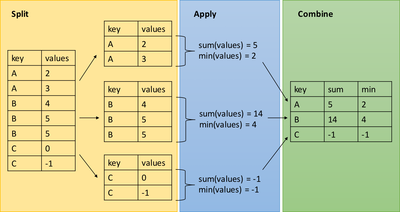
The dplyr verbs become especially powerful when they are are combined using the pipe operator |>.
The following dplyr functions allow us to split our data frame into groups on which we can perform operations individually
group_by(): group data frame by a factor for downstream operations (usually summarise)
summarise(): summarise values in a data frame or in groups within the data frame with aggregation functions (e.g. min(), max(), mean(), etc…)

`dplyr` - Split-Apply-Combine

The group_by function is key to the Split-Apply-Combine strategy

The `summarize()` function

The summarize() function is used in the R program to summarize the data frame into just one value or vector.
This summarization is done through grouping observations by using categorical values at first, using the group_by() function.
The summarize() function offers the summary that is based on the action done on grouped or ungrouped data.

`dplyr::summarize()` Function

To calculate the mean bmi in base R vs with summarize()::

Code

mean(yrb_data$bmi, na.rm = T)

[1] 23.49541

summarize(new_column = summary_function(column))

Code

yrb_data %>% filter(!is.na(bmi)) %>% 
  summarize(mean_bmi = mean(bmi))

# A tibble: 1 × 1
  mean_bmi
     <dbl>
1     23.5

Multiple Summary Statistics

You can calculate multiple statistics in one summarize():

Code

yrb_data %>% filter(!is.na(bmi)) %>% 
  summarize(mean_age = mean(bmi), 
            median_bmi = median(bmi))

# A tibble: 1 × 2
  mean_age median_bmi
     <dbl>      <dbl>
1     23.5       22.3

Grouped summaries with `dplyr::group_by()`

group_by() groups data by one or more variables.

Example 1: Mean Age by Sex

Code

yrb_data %>% 
  group_by(sex)

Result: Different mean ages for each group (e.g., male and female).

Example 2: Maximum and Minimum Weights

Calculate the max and min weights for each sex:

Code

yrb_data %>% 
  group_by(sex) %>% filter(!is.na(stweight)) %>% 
  summarize(max_weight = max(stweight), 
            min_weight = min(stweight))

# A tibble: 2 × 3
  sex    max_weight min_weight
  <chr>       <dbl>      <dbl>
1 Female       181.       27.7
2 Male         181.       35.4

Why `summarize()` Matters

The combination of group_by() and summarize() allows highly informative grouped summaries of datasets with minimal code.
- Producing such summaries is an essential data analysis skill.

Grouping by Multiple Variables (Nested Grouping)

To group by more than one variable, list both in group_by():

Code

yrb_data %>% group_by(sex, grade) %>% filter(!is.na(bmi)) %>%   
  summarize(mean_bmi = mean(bmi)) %>% head(4)

# A tibble: 4 × 3
# Groups:   sex [1]
  sex    grade mean_bmi
  <chr>  <chr>    <dbl>
1 Female 10th      23.0
2 Female 11th      23.4
3 Female 12th      23.9
4 Female 9th       22.8

You can swap the column order in group_by():

Code

yrb_data %>% group_by(grade, sex) %>% filter(!is.na(bmi)) %>%    
  summarize(mean_bmi = mean(bmi)) %>% head(4)

# A tibble: 4 × 3
# Groups:   grade [2]
  grade sex    mean_bmi
  <chr> <chr>     <dbl>
1 10th  Female     23.0
2 10th  Male       23.5
3 11th  Female     23.4
4 11th  Male       24.1

Ungrouping Data

After group_by() and summarize(), the resulting data frame may still be grouped.
To avoid unintended behaviors, use ungroup():

Code

yrb_data %>% group_by(sex, grade) %>%   
  summarize(mean_bmi = mean(bmi)) %>% ungroup() %>% head()

# A tibble: 6 × 3
  sex    grade mean_bmi
  <chr>  <chr>    <dbl>
1 Female 10th        NA
2 Female 11th        NA
3 Female 12th        NA
4 Female 9th         NA
5 Female <NA>        NA
6 Male   10th        NA

Why is `ungroup()` Needed?

Grouped data frames behave uniquely with other dplyr functions like select(), filter(), or mutate():

Code

# Unexpected behavior when grouped 
yrb_data %>% group_by(sex, grade) %>% filter(!is.na(bmi)) %>%    
  summarize(mean_bmi = mean(bmi)) %>% select(mean_bmi) %>% head(4)

# A tibble: 4 × 2
# Groups:   sex [1]
  sex    mean_bmi
  <chr>     <dbl>
1 Female     23.0
2 Female     23.4
3 Female     23.9
4 Female     22.8

By ungrouping, we get the expected output:

Code

yrb_data %>% group_by(sex, grade) %>% filter(!is.na(bmi)) %>% 
  summarize(mean_bmi = mean(bmi)) %>%   
  ungroup() %>% select(mean_bmi) %>% head(3)

# A tibble: 3 × 1
  mean_bmi
     <dbl>
1     23.0
2     23.4
3     23.9

Counting Rows

Use n() inside summarize() to count rows:

Code

yrb_data %>%    
  group_by(sex) %>%    
  summarize(count = n())

# A tibble: 3 × 2
  sex    count
  <chr>  <int>
1 Female  9592
2 Male   10177
3 <NA>     231

You can combine counts with other summary statistics:

Code

yrb_data %>%    
  group_by(sex) %>%    
  summarize(count = n(), 
            mean_bmi = mean(bmi, na.rm=T))

# A tibble: 3 × 3
  sex    count mean_bmi
  <chr>  <int>    <dbl>
1 Female  9592     23.3
2 Male   10177     23.7
3 <NA>     231    NaN

Counting Rows with Conditions

To count rows that meet specific conditions, wrap the condition in sum():

Code

yrb_data %>% group_by(race7) %>% filter(!is.na(bmi)) %>%  
  summarize(count_above50 = sum(bmi > 50))

# A tibble: 8 × 2
  race7                     count_above50
  <chr>                             <int>
1 Am Indian / Alaska Native             1
2 Asian                                 1
3 Black or African American             7
4 Hispanic/Latino                       2
5 Multiple - Non-Hispanic               3
6 Native Hawaiian/other PI              1
7 White                                 2
8 <NA>                                  0

For binary variables, TRUE equals 1, and FALSE equals 0, making sum() work seamlessly.

Counting Missing Values

To count NAs:

Code

yrb_data %>% group_by(sex) %>% 
  summarize(unknown_bmi = sum(is.na(bmi)))

# A tibble: 3 × 2
  sex    unknown_bmi
  <chr>        <int>
1 Female        2970
2 Male          3257
3 <NA>           231

To count known (non-missing) values:

Code

yrb_data %>%    group_by(sex) %>%    
  summarize(known_bmi = sum(!is.na(bmi)))

# A tibble: 3 × 2
  sex    known_bmi
  <chr>      <int>
1 Female      6622
2 Male        6920
3 <NA>           0

Using `dplyr::count()`

count() simplifies counting observations by group:

Code

yrb_data %>% count(race4)

# A tibble: 5 × 2
  race4                         n
  <chr>                     <int>
1 All other races            4713
2 Black or African American  4093
3 Hispanic/Latino            4670
4 White                      5814
5 <NA>                        710

This is equivalent to:

Code

yrb_data %>% group_by(race4) %>%    
  summarize(n = n())

# A tibble: 5 × 2
  race4                         n
  <chr>                     <int>
1 All other races            4713
2 Black or African American  4093
3 Hispanic/Latino            4670
4 White                      5814
5 <NA>                        710

You can count by multiple variables:

Code

yrb_data %>% count(sex, grade)

# A tibble: 15 × 3
   sex    grade     n
   <chr>  <chr> <int>
 1 Female 10th   2332
 2 Female 11th   2365
 3 Female 12th   2277
 4 Female 9th    2492
 5 Female <NA>    126
 6 Male   10th   2539
 7 Male   11th   2496
 8 Male   12th   2263
 9 Male   9th    2684
10 Male   <NA>    195
11 <NA>   10th     36
12 <NA>   11th     30
13 <NA>   12th     37
14 <NA>   9th      43
15 <NA>   <NA>     85

`count()` vs. `summarize()`

The count() function is limited to row counts, while summarize() can produce multiple summary statistics:

Code

yrb_data %>%    group_by(sex, grade) %>%    
  summarize(count = n(), median_bmi = median(bmi)) %>% head()

# A tibble: 6 × 4
# Groups:   sex [2]
  sex    grade count median_bmi
  <chr>  <chr> <int>      <dbl>
1 Female 10th   2332         NA
2 Female 11th   2365         NA
3 Female 12th   2277         NA
4 Female 9th    2492         NA
5 Female <NA>    126         NA
6 Male   10th   2539         NA

Summarize grouped data

The operations that can be performed on grouped data are average, factor, count, mean, etc.
Example: we are interested in the mean temperature and standard deviation within each month of the airquality dataset

Code

month_sum <- airquality |>
      group_by(Month) |>
      summarise(mean_temp = mean(Temp),
                sd_temp = sd(Temp))
month_sum

# A tibble: 5 × 3
  Month mean_temp sd_temp
  <int>     <dbl>   <dbl>
1     5      65.5    6.85
2     6      79.1    6.60
3     7      83.9    4.32
4     8      84.0    6.59
5     9      76.9    8.36

Summarize ungrouped data

We can also summarize ungrouped data. This can be done by using three functions.
- summarize_all()
- summarize_at()
- summazrize_if()

1. summarize_all()

This function summarizes all the columns of data based on the action which is to be performed. summarize_all(action)
example The code airquality |> summarize_all(mean) will show the mean of all columns.

Code

# Caculating mean value.
airquality |> summarize_all(mean, na.rm=T)

     Ozone  Solar.R     Wind     Temp    Month      Day
1 42.12931 185.9315 9.957516 77.88235 6.993464 15.80392

2. summarize_at()

It performs the action on the specific column and generates the summary based on that action.
summarize_at(vector_of_columns, action)
vector_of_columns: The list of column names or character vector of column names.

Code

airquality |> group_by(Month) |>
summarize_at(c("Wind","Temp"),mean)

# A tibble: 5 × 3
  Month  Wind  Temp
  <int> <dbl> <dbl>
1     5 11.6   65.5
2     6 10.3   79.1
3     7  8.94  83.9
4     8  8.79  84.0
5     9 10.2   76.9

3. summarize_if()

In this function, we specify a condition and the summary will be generated if the condition is satisfied.

Code

summarize_if(.predicate, .action)

In the code snippet below, we use the predicate function is.numeric and mean as an action.

Code

airquality |> group_by(Month) |>
summarize_if(is.numeric, mean)

# A tibble: 5 × 6
  Month Ozone Solar.R  Wind  Temp   Day
  <int> <dbl>   <dbl> <dbl> <dbl> <dbl>
1     5    NA     NA  11.6   65.5  16  
2     6    NA    190. 10.3   79.1  15.5
3     7    NA    216.  8.94  83.9  16  
4     8    NA     NA   8.79  84.0  16  
5     9    NA    167. 10.2   76.9  15.5