Yebelay Berehan – Introduction to R and RStudio

Introductions

Take few minutes to introduce ourselves.

Please share …

Your name
Your experience in R
What you expect at end of the training

30:00

Outlines

01. Module 1

Overview of R and R Studio
Workspace and R Objects
Reading and Writing data

02. Module 2

The Tidyverse
- Data Manipulation
- Reshaping data
Recoding Variables
Data mergining
Data cleaning

03. Module 3

Data visualization
Working with factors using forcats

04. Module 4

Creating reproducible reports
Statistical Analysis

Getting started

Learn objectives

Be able to setting up and utilizing R & RStudio
Navigating R & Rmarkdown scripts and RStudio projects
Basic operations in R/RStudio
Be able to importing and inspecting data sets in R
Understand data structures
Know how to get help
Manipulating data through filtering, summarizing, transforming, and joining
Visualizing data using the renowned ggplot2 package

1. Why R?

It is free, versatile, fast, and modern.
It has a large and friendly community of users.
With more than 22,000 add-on packages available, R offers more functions for data analysis than any other statistical software.
R makes it easy to construct reproducible analyses and workflows that allow you to easily repeat the same analysis more than once.
It is flexible enough to be used to create interactive web pages (eg. my draft website) and automated reports.
Simply currently the best tool there is for data analysis.

What are Advantages or Disadvantages of R

Advantages

Availability and compatibility
State of the art graphics capabilities
Can import files from other (statistical) programs
New version every x months
Interactive development environments (IDEs) available
Large users community
reproducible research

Drawbacks of R

Expert friendly
Learn by example
Not very (easily) interactive
Command based
Documentation sometimes cryptic
(Too) large amount of resources
Constantly evolving
Memory intensive and slow at times

2. RStudio

What is RStudio? Why use it?

Best Integrated Development Environment (IDE) for R.
Powerful and makes using R easier
RStudio can:
- Organize your code, output, and plots.
- Auto-complete code and highlight syntax.
- Help view data and objects.
- Enable easy integration of R code into documents.
User-friendly interfaces
R is like a car’s engine
Rstudio is like a car’s dashboard

Set up on Windows

Follow the steps below to download and install R:

Go to cran.rstudio.com to access the R installation page. Then click the download link for Windows:
Choose the base sub-directory.
Then click on the download link at the top of the page to download the latest version of R:

During installation, accept the defaults; just keep clicking Next until the installation is done.

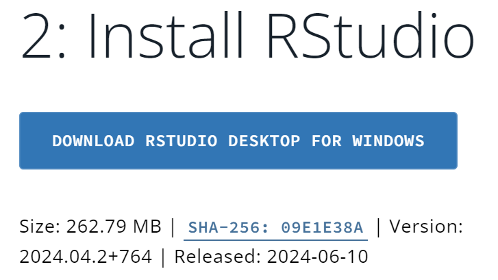
Download, install & run RStudio

To download RStudio,
- posit.co/download/rstudio-desktop and download the Windows version.
Then click on the downloaded file and follow the installation instructions.

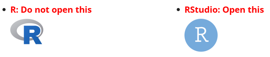
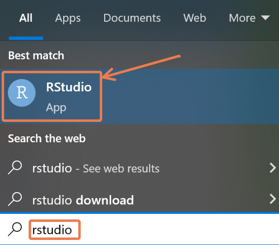
Now click to open the app from the start menu:

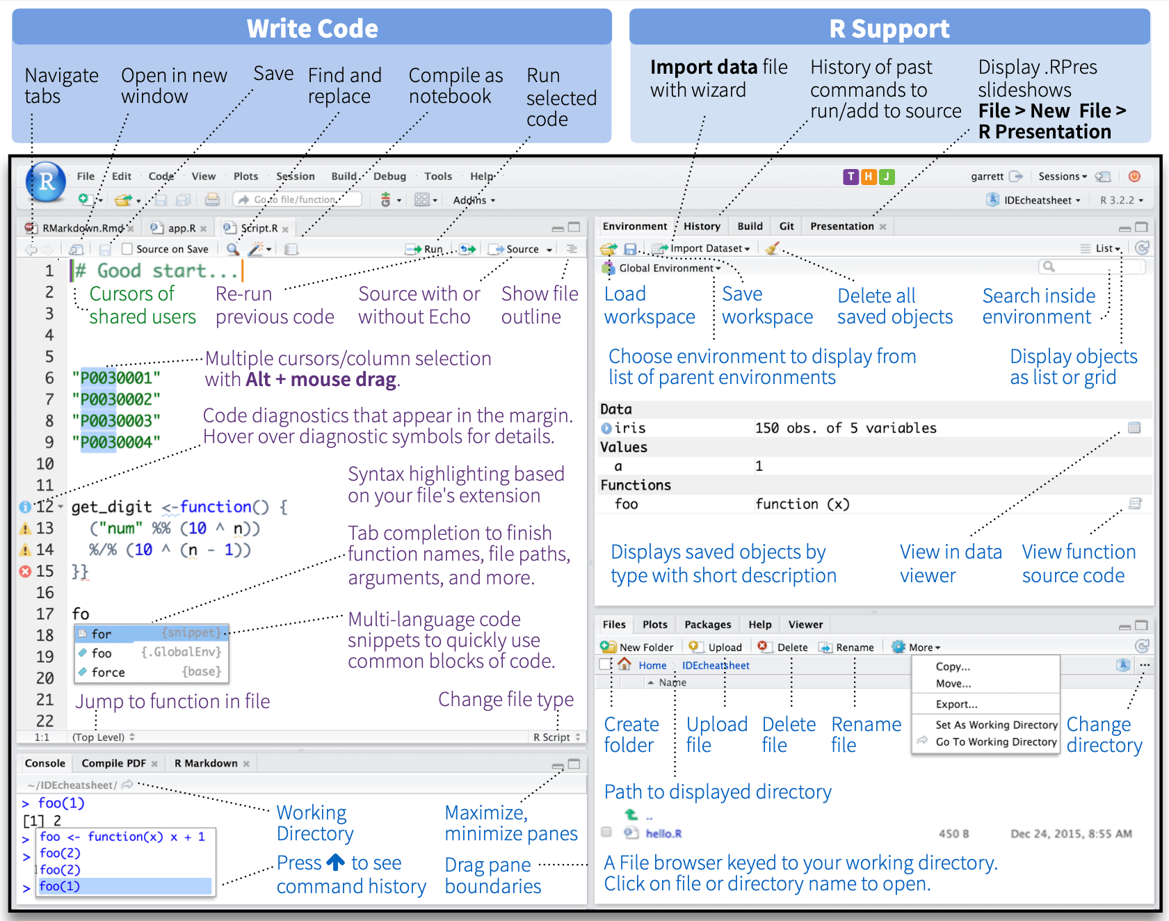
RStudio Overview

Getting Started

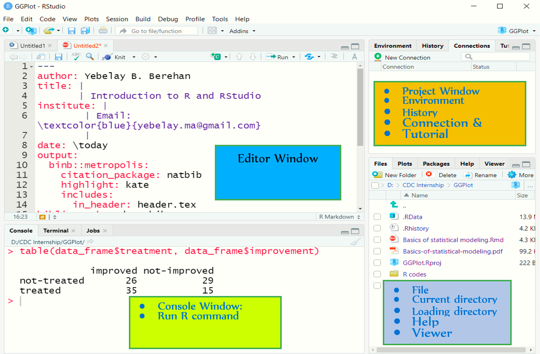
RStudio will open with 4 sections (called panes):

1. Source editor pane

You will write your R code/script here and it will be run in the console.
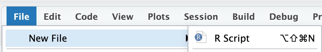
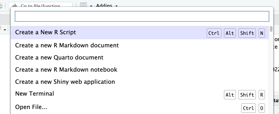
To create a new R script you can either go to File -> New -> R Script, or click on the icon with the + sign and select R Script, or simply press Ctrl+Shift+N.
Make sure to save the script.

2. Console pane

Interactively run R commands

3. Environment/history pane

Environment: view objects in the global environment
History: search and view command history

4. Files/Plots/Packages/Help pane

Files: navigate directories and
Plots: view generated plots.
Packages: manage packages (install or update)
Help: View help documentations for any package/function

Customization

Panes

The size and position of the panes can be customized.
On the top right of each pane, there are buttons to adjust the pane size.
Also, place your mouse pointer/cursor on the borderline between panes and when the pointer changes its shape, click and drag to adjust the pane size.
For more options, go to View > Panes on the menu bar.
Alternatively, try Tools > Global Options > Pane Layout.

Appearances

The overall appearance can be customized as well.
Go to Tools > Global Options> Appearance on the menu bar to change themes, fonts, and more.

The RStudio panes

By default, RStudio is arranged into four window panes.
If you only see three panes, open a new script with File > New File > R Script . This should reveal one more pane.

Before we go any further, we will rearrange these panes to improve the usability of the interface.
Then under Pane Layout, adjust the pane arrangement. The arrangement we recommend is shown below.

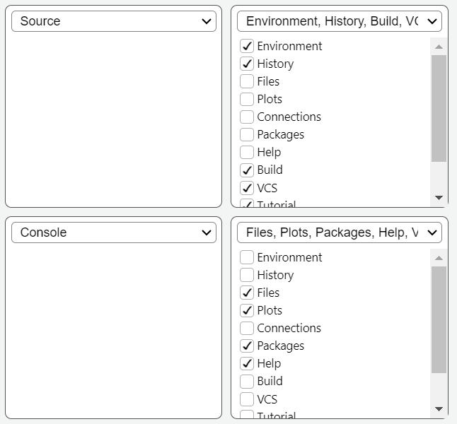
The RStudio panes

At the top left pane is the Source tab, and at the top right pane, you should have the Console tab.
Then at the bottom left pane, no tab options should checked—this section should be left empty, with the drop-down saying just “TabSet”.
Finally, at the bottom right pane, you should check the following tabs: Environment, History, Files, Plots, Packages, Help and Viewer.

The RStudio panes

First, open a new script under the File menu if one is not yet open: File > New File > R Script. In the script, type the following:

Code

print("excited for R!")

To run code, place your cursor anywhere in the code, then hit Control + Enter on Windows.
This should send the code to the Console and run it.

You can also run multiple lines at once.

Code

print("excited for R!")
print("and RStudio!")

Now drag your cursor to highlight both lines and press Control + Enter.
To run the entire script, you can use Control + A to select all code, then press `Control + Enter.

The RStudio panes

To open the script in a new window, click on the third icon in the toolbar directly above the script.

To put the window back, click on the same button on the now-external window.
Next, save the script. Hit Control + S to bring up the Save dialog box.

Console

The console, at the bottom left, is where code is executed. You can type code directly here, but it will not be saved.
Type a random piece of code (maybe a calculation like 3 + 3) and press ‘Enter’.

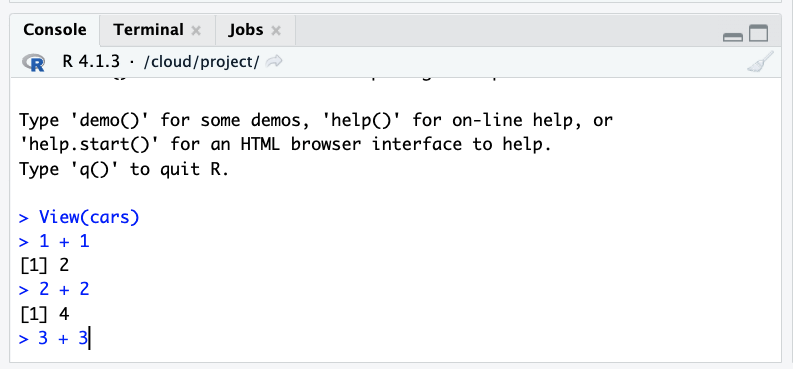
If you place your cursor on the last line of the console, and you press the up arrow, you can go back to the last code that was run. Keep pressing it to cycle to the previous lines.
To run any of these previous lines, press Enter.

Environment

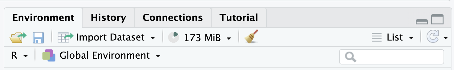
At the top right of the RStudio Window, you should see the Environment tab.
The Environment tab shows datasets and other objects that are loaded into R’s working memory, or “workspace”.
To explore this tab, let’s import a dataset into your environment from R.
Type the code below into your script and run it:

Code

data <- iris

You have now imported the dataset and stored it in an object named data. (You could have named the object anything you want.)

Environment

Now that the dataset is stored by R, you should be able to see it in the Environment pane.
If you click on the blue drop-down icon beside the object’s name in the Environment tab to reveal a summary.

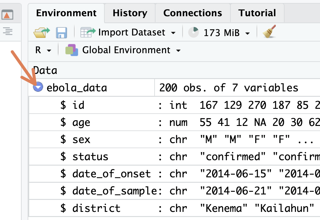
Try clicking directly on the data dataset from the Environment tab. This opens it in a ‘View’ tab.

Environment

The broom icon, at the top of the Environment pane is used to clear your workspace.

You can also remove an object from the workspace with the rm() function.
Type and run the following in a new line on your R script.

Code

rm(data)

Notice that the data object no longer shows up in your environment after having run that code.

History

Next, the History tab shows previous commands you have run.

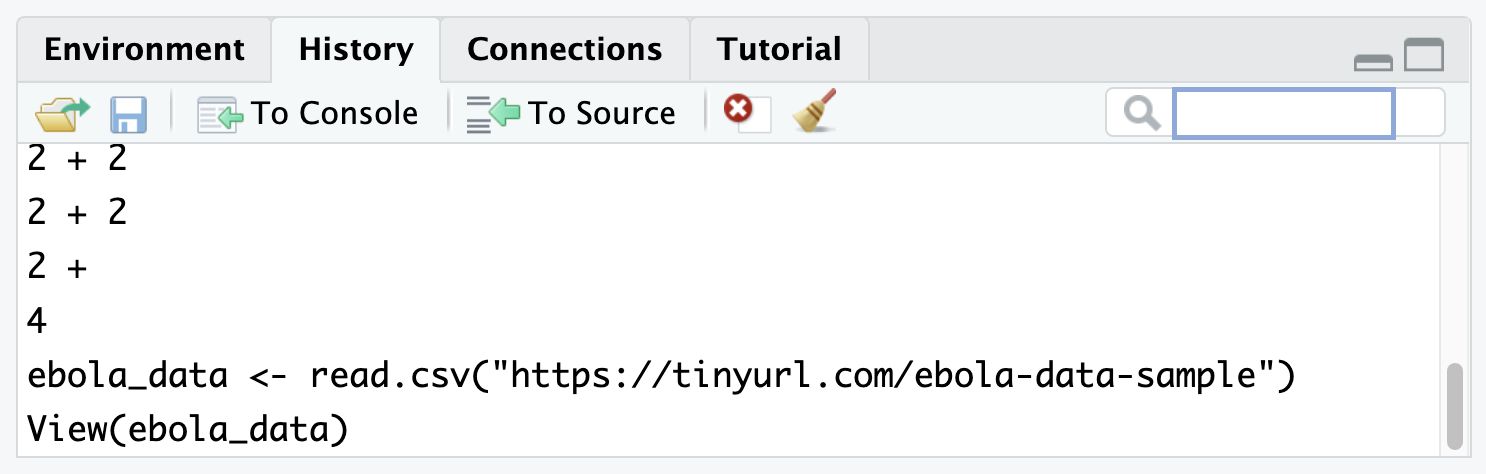
You can click a line to highlight it, then send it to the console or to your script with the “To Console” and “To Source” icons at the top of this tab.
To select multiple lines, use the “Shift-click” method: click the first item you want to select, then hold down the “Shift” key and click the last item you want to select.
Finally, notice that there is a search bar at the top right of the History pane where you can search for past commands that you have run.

Files

Next, the Files tab. This shows the files and folders in the folder you are working in.

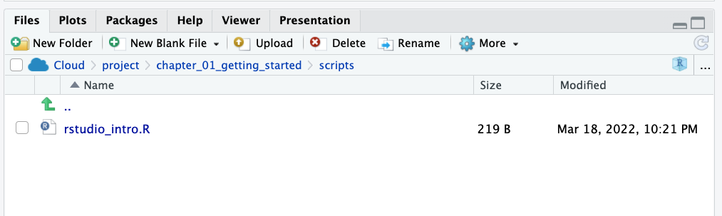
The tab allows you to interact with your computer’s file system.
Try playing with some of the buttons here, to see what they do. You should try at least the following:
- Make a new folder
- Delete that folder
- Make a new R Script
- Rename that script

Plots

Next, the Plots tab. This is where figures that are generated by R will show up.
Try creating a simple plot with the following code:

Code

plot(women)

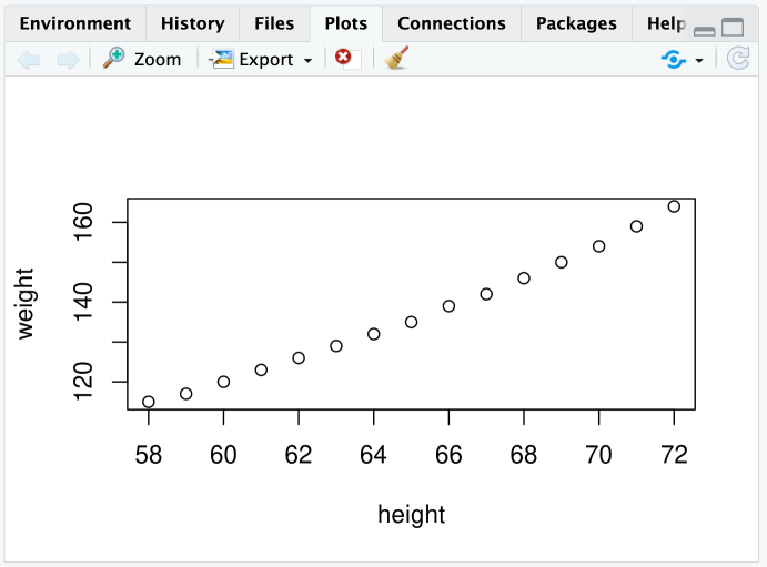
That code creates a plot of the two variables in the women dataset.
You should see this figure in the Plots tab.
Now, test out the buttons at the top of this tab to explore what they do.
In particular, try to export a plot to your computer.

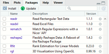
Packages

Next, let’s look at the Packages tab.

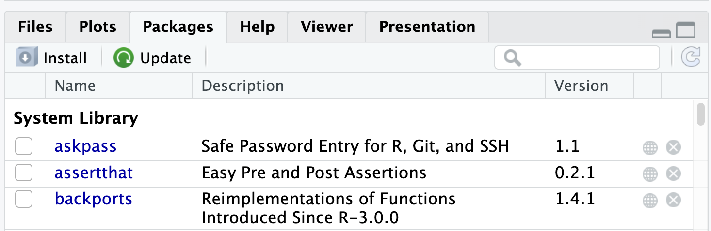
Packages are collections of R code that extend the functionality of R.
it is important to know that to use a package, you need to install then load it.
Packages need to be installed only once, but must be loaded in each new R session.
All the package names you see (in blue font) are packages that are installed on your system. And packages with a checkmark are packages which are loaded in the current session.
Best resourse showing how to adjust panels, personalize how Rstudio looks, etc

Installing and Loading Packages

Packages are collections of R functions, data, and compiled code in a well-defined format.
There are three categories of packages.

1. Base Packages: Providing the basic functionality, maintained by the R Core Development group. Currently, there are 14 packages, these are

Code

rownames(installed.packages(priority="base"))

 [1] "base"      "compiler"  "datasets"  "graphics"  "grDevices" "grid"     
 [7] "methods"   "parallel"  "splines"   "stats"     "stats4"    "tcltk"    
[13] "tools"     "utils"

2. Recommended Packages: also a default package, mainly including additional more complex statistical procedures. These are 15 packages

Code

rownames(installed.packages(priority="recommended"))

 [1] "boot"       "class"      "cluster"    "codetools"  "foreign"   
 [6] "KernSmooth" "lattice"    "MASS"       "Matrix"     "mgcv"      
[11] "nlme"       "nnet"       "rpart"      "spatial"    "survival"

3. Contributed packages: Due to the open nature of R, anyone can contribute new packages at any time.

Currently, the CRAN package repository features 20394 available packages.

Code

nrow(available.packages())

Installing Packages

Option 1: Menu

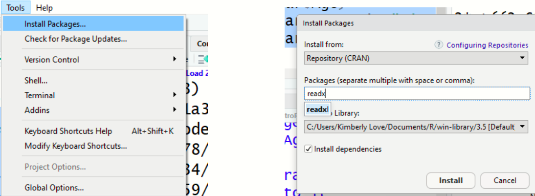
Option 2: Packages Window

Option 3: Code

Code

install.packages("readxl")

Loading Packages

Code

library()   # see all packages installed
search()    # see packages currently loaded

Updating R and RStudio

Updating R

Go to CRAN and download new version
More efficient: install installr package, load it, and run updateR()
- Updates R and Optionally updates all packages
- May be better to do this in basic Rgui
Version should update automatically in RStudio
- Check/change R version under [Tools>Global Options>R version]{style=“color:green”}
Then update the R packages with the code:

Code

update.packages(ask = FALSE, checkBuilt = TRUE)

To updating RStudio: Go to RStudio and download new version
Click on Help>Check for Updates, follow menu prompts

Viewer

Notice that the histogram above shows up in a Viewer tab. This tab allows you to preview HTML files and interactive objects.

Help

Lastly, the Help tab shows the documentation for different R objects. Try typing out and running each line below to see what this documentation looks like.

Code

?hchart
?women
?read.csv

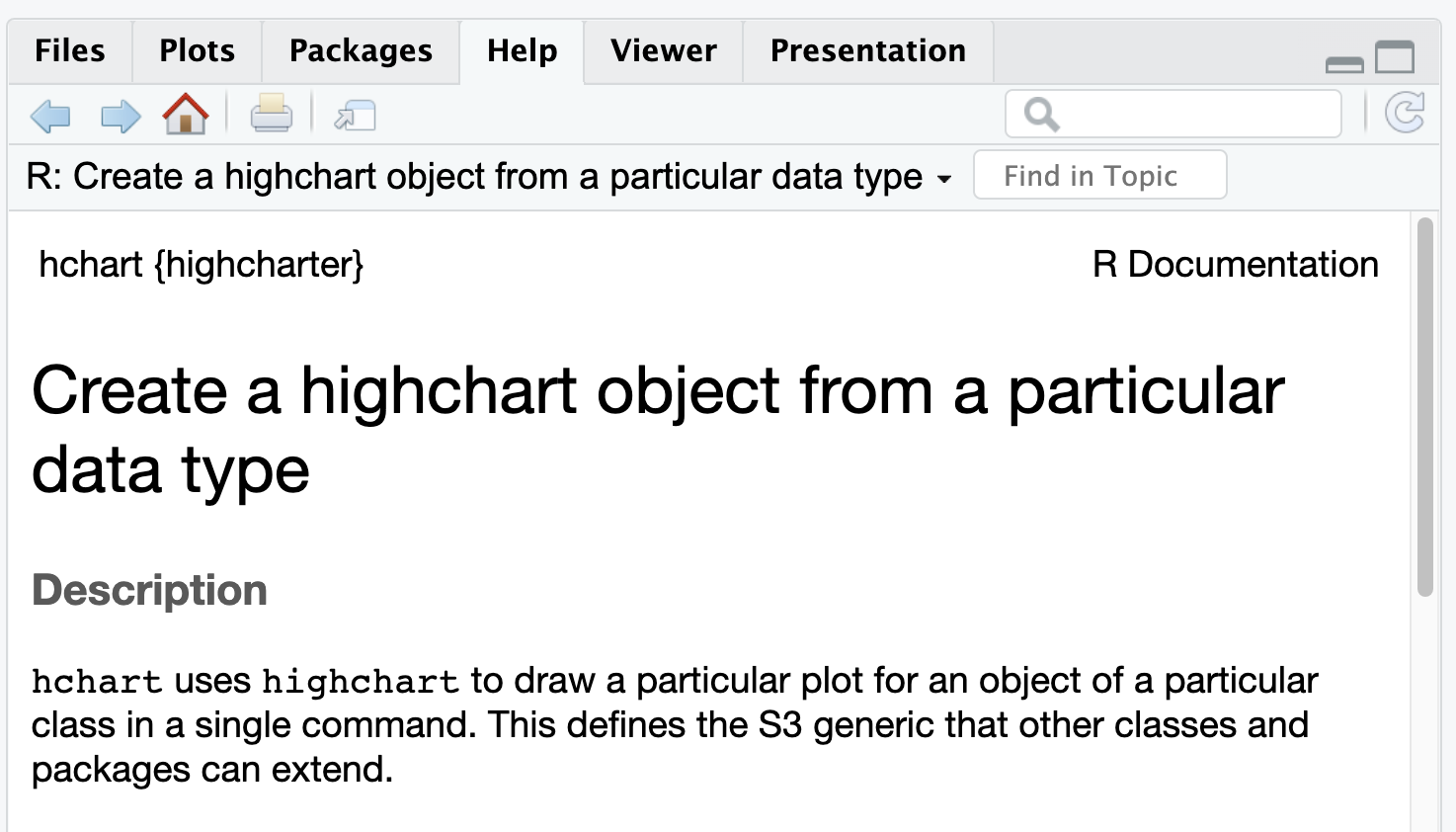
Help files are not always very easy to understand for beginners, but with time they will become more useful.

RStudio options

RStudio has a number of useful options for changing it’s look and functionality. Let’s try these.
You may not understand all the changes made for now. That’s fine.
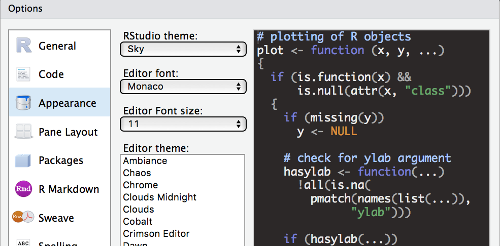
In the RStudio menu at the top of the screen, select Tools > Global Options to bring up RStudio’s options.
Now, under Appearance, choose your ideal theme. (We like the “Crimson Editor” and “Tomorrow Night” themes.)

RStudio options

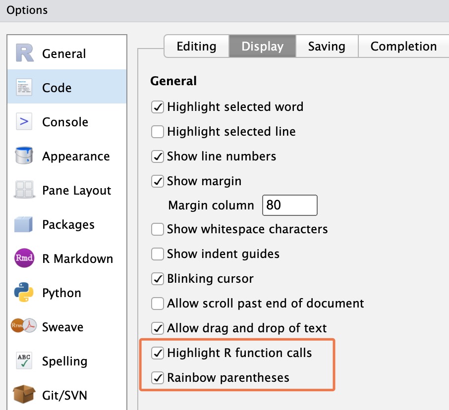
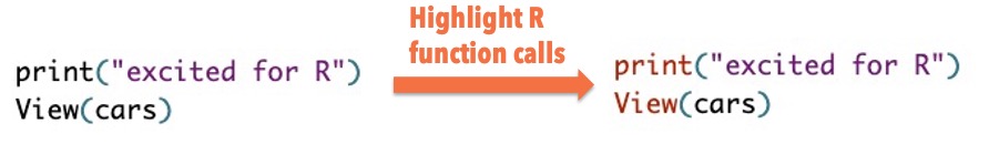
Under Code > Display, check “Highlight R function calls”.
What this does is give your R functions a unique color, improving readability.
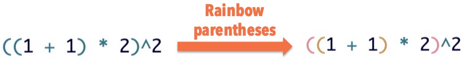
Also under Code > Display, check “Rainbow parentheses”.
What this does is make your “nested parentheses” easier to read by giving each pair a unique color.

RStudio options

Finally under General > Basic, uncheck the box that says “Restore .RData into workspace at startup”.
You don’t want to restore any data to your workspace (or environment) when you start RStudio.
Starting with a clean workspace each time is less likely to lead to errors.
This also means that you never want to “save your workspace to .RData on exit”, so set this to Never.

Command palette

The Rstudio command palette gives instant, searchable access to many of the RStudio menu options and settings that we have seen so far.
The palette can be invoked with the keyboard shortcut Ctrl + Shift + P.
It’s also available on the Tools menu (Tools -> Show Command Palette).

Try using it to:

Create a new script (Search “new script” and click on the relevant option)
Rename a script (Search “rename” and click on the relevant option)

Wrapping up

Of course, you have only scratched the surface of RStudio functionality and you can find more on the cheatsheet below:

3. Working with R Objects

R Projects (why .Rproj file?) & Good Practices

The workspace is a working environment where R will store and remember user-defined objects: vectors, matrices, data frames, lists, variables, etc.
Use projects to keep everything together
Create an RStudio project foreach data analysis project, for each homework assignment, etc.
A project is associated with a directory folder
- Keep data files there
- Keep scripts there; edit them, run them in bits or as a whole
- Save your outputs (plots and cleaned data) there
Only use relative paths, never absolute paths
- relative (good): read.csv("data/mydata.csv")
- absolute (bad): read.csv("/home/yourname/Documents/stuff/mydata.csv")

Advantages of using projects

standardizes file paths
keep everything together
a whole folder can be easily shared and run on another computer
when you open the project everything is as you left it
To Create an R project, go to
- File \> New Project and then choose: New Directory\> Name for the directory \> Click on Create Project
For more complex projects it may be useful to create sub-directories to contain data, scripts, and other documents separately.
You can also type the below function into the Console, but we won’t do that in this session.

Code

prodigenr::setup_project("C:/Users/YebelayBerehan/Downloads/LearningR")

Objects in R

R is an object-oriented programming platform.
Meaning the entities that R creates and manipulates are known as objects.
During an R session, objects are created and stored by name.

Code

objects() # lists all objects
ls() # lists all objects alternatively
rm(x) #removes an object

Objects can be created in the form of
- variable <- value or variable = value or variable -> value.
- Variable names can be letters, numbers, and the dot or underline characters but not dot followed by numbers .4youis illegal).

Objects in R

the symbol <- (Alt + -) that could be read as assign or place into or read in etc.

Code

# need to placed in quotes as diabetic is string.
A <-"Diabetic"#<<

The standard data objects in R are:
- scalars and vectors,
- factors,
- matrices and arrays,
- lists, and
- data frames.

Data typesassigned to each objects are:
- logical,
- numeric,
- integer,
- character

Vector

A set of scalars arranged in a one-dimensional array.
Data values are all the same mode(data type), but can hold any mode.
- e.g:(-2, 3.4, 3), (TRUE, FALSE, TRUE), (“blue”, “gray”, “red”)
Vectors can be created using the following functions:
c() function to combine individual values
- x <- c(10.4, 5.6, 3.1, 6.4, 21.7)
seq() to create more complex sequences
- seq(from=1, to=10, by=2) or seq(1,10 )
rep() to create replicates of values: rep(1:4, times=2, each=2)

Some useful functions in vector

class(x): returns class/type of vector x
length(x): returns the total number of elements
x[length(x)]: returns last value of vector x
rev(x): returns reversed vector
sort(x): returns sorted vector
unique(x): returns vector without multiple elements
range(x): Range of x
quantile(x): Quantiles of x for the given probabilities
which.max(x): index of maximum
which.min(x): index of minimum

Factors

A factor is used to store predefined categorical data
Can be ordered and unordered
- e.g. :(“yes”, “no”, “no”, “yes”, “yes”), (“male”, “female”, “female”, “male”)
Factors can be created using factor()

Code

size <- factor(c("small", "large", "small", "medium"))

The levels of a factor can be displayed using levels().

Matrix

Matrix is a rectangular array arranged in rows and columns.
The individual items in a matrix are called its elements or entries.
Matrices can be created by:

matrix()
converting a vector into a matrix
binding together vectors

Matrices can be created using the functions:
- matrix() creates a matrix by specifying rows and columns
- dim() sets dimensions to a vector
- cbind combines columns
- rbind combines rows

Matrix

e.g.

Code

m1<-matrix(data = 1:6, nrow = 3, ncol = 2)
m2<-cbind(1:3,5:7,10:12)
x=1:6
dim(x) <- c(2, 3)

Note: dim() can also be used to retrieve dimensions of an object!

Assign names to rows and columns of a matrix

Code

rownames(m1) <- c("A", "B", "C") 
colnames(m1)<- c("a","b")

Data frames

a data set in R is stored a data frame.
Two-dimensional, arranged in rows and columns created using the function: data.frame()
e.g.

Code

df <- data.frame(ID = 1:3, Sex = c("F", "F", "M"), Age = c(17, 18,18))

We can enter data directly by access the editor using either the edit() or fix()

Code

 new.data<-data.frame()  # creates an "empty" data frame
 new.data<-edit(new.data) # request the changes or  `fix(new.data)`

We’ll use the data set called iris data to do this exploration.

Code

library(readr)
data <- read_csv("iris.csv")
#View(data)

Some functions for inspecting the data

Use head() and tail() to view the first (and last) five rows
Use View() to view an entire data.table object
Use str() to view the structure of data.table object
Use tables() to show all loaded data.table objects
Use colnames() or names() to look variable names
Use colSums(is.na()) to sum missing data
Use subset() to subset data.
Use attributes() to look attributes of the dataframe
Use dim() or ncol() and nrow() to see dimensions of the dataframe
Use summary() to see basic statistics for each variables

Subsetting

Code

iris[] # the whole data frame 
iris[1, 1] # 1st element in 1st column 
iris[1, 6] # 1st element in the 6th column 
iris[, 1] # first column in the data frame 
iris[1] # first column in the data frame 
iris[1:3, 3] 
iris[3, ] # the 3rd row 
iris[1:6, ] # the 1st to 6th rows
iris[c(1,4), ] # rows 1 and 4 only 
iris[c(1,4), c(1,3) ] 
iris[, -1] # the whole except first column
iris$Variable1 # Also extracts the first column
iris[,c("col3", "col4")]# extract by name of column

4. Reading and Writing data

Importing data is rather easy in R but that may also depend on the nature of the data to be imported and from what format.
Most data are in tabular form such as a spreadsheet or a comma-separated file (.csv).
Base R has a series of read functions to import tabular data from plain text files with columns delimited by: space, tab, and comma, with or without a header containing the column names.
With an added package it is also possible to import directly from a Microsoft Excel spreadsheet format or other foreign formats from various sources.

Importing from local files

In base R the standard commands to read text files are based on the read.table()function.
The following table lists the collection of the base R read functions.
For more details use the help command help(read.table) that will display help for all.

Details of dataset readings
Function name	Assumes header	Separator	Decimal	File type
read.table()	No	” ”	.	.text
read.csv()	Yes	“,”	.	.csv
read.csv2()	Yes	“;”	,	.csv
read.delim()	Yes	“tab”	.	.text
read.delim2()	Yes	“tab”	,	.text

Reading raw data from other sources

Import data

There are many ways to get data into R and out of R.
Import text file data using read.table() and comma separated files using read.csv() functions.

Code

# syntax: 
read.table("file name with full path", arguments)#<<

Code

# Examples:# Creates a data frame named myData
  mydata<- read.table(file = "datafile.txt",sep=" ", header=TRUE)
  mydata<- read.csv(file = "datafile.csv")

File names are specified in the same way as file.choose() function can be used to select the file interactively. i.e.

Code

mydata <-read.csv(file.choose(),sep=",",header=T)

Reading raw data from other sources

Useful arguments - Check these arguments carefully when you load your data

Code

myData<-read.csv(file="datafile.csv",header= TRUE, sep=",", strip.white =TRUE,
                 na.strings= " ")

You can reduce possible errors when loading a data file
The header = TRUE argument tells R that the first row of your file contains the variable names
The sep = "," argument tells R that fields are separated by comma
The strip.white = TRUE argument removes white space before or after factors that has been mistakenly inserted during data entry.
The na.strings = " " argument replaces empty cells by NA (missing data in R)

Read data

Stata to R: Different packages for stata version >=13 vs. <13

Code

library(foreign) # Versions before stata 13
data <-  read.dta(file="XXX.dta") # Other options

Code

library(readstata13) # Versions from stata 13
data <-  read.dta13(file="XXX.dta") # Other options

Excel to R: There are several packages

Code

library(readxl)
data <-  read_xlsx(path="XXX.xlsx", sheet = 1, col_names = TRUE)

Code

library(readr)
data <- read_csv("path=XXX.csv")

Read data

CSV to R: There are several packages

Code

library(readr)
data <- read_csv(file="XXX.csv")

Text file to R: Available in R base, used for text and csv files

Code

data <- read.table(file="XXX.txt",header=TRUE, sep="")

Code

data <- read.table(file="XXX.csv",header=TRUE, sep=",")

Data import wizard

The data import wizard is a quick and easy way to import your data

It’s actually way better to follow the reproducible steps – and hardly any more effort – below…

Inside the data wizard, you can copy the code int he code-preview window, then paste the code into the code chunk of your quarto document or r script.

Code

# library(readr)
#brodhead_center <- read_csv("data/brodhead_center.csv")
# view(brodheadCenter)

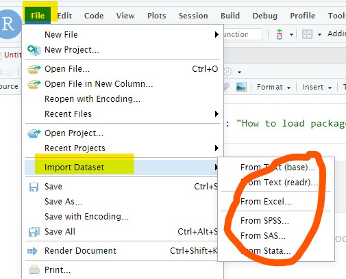
Composing the data import code…

Writing the import data function can be tricky. Try the import wizard pictured above. THEN, paste the code from the Code Preview section into your script.

Excel, SPSS, SAS, etc.

The data import wizard will help you find the proper package for importing your data. For example, use…

library(readxl) for Excel data
library(haven) for SPSS, SAS, Stata
lirary(readr) for CSV or other delimeters

Just start with File > Import Dataset to get started composing that code, then paste your code into a script.

Exporting Data

R to Stata: Use the libraries haven or readstata13

Code

write.dta(data,file="XXX.dta")# Other options
save.dta13(data, file="XXX.dta") # Other options

R to Excel: Note the package readxl does not work here

Code

library(xlsReadWrite)
write.xls(data,"data.xls")# Other options

R to csv: Use readr package

Code

write_csv(data, "data.csv", na = "")

R to a text file:

Code

write.table(data, "data.txt", sep="\t")