Data Management

Using an Ethiopian Malaria Indicator Survey data

Yebelay & Leyikun

Ethiopian Public health Institute (EPHI)

2026-06-18

Data Manipulation and Cleaning using `dplyr()` package

What is Tidyverse?

The tidyverse library is a collection of several R packages that are designed to work together to make data manipulation and visualization tasks easier.
a suite of packages that implement tidy methods for data importing, cleaning, and wrangling.
Contains a series of packages useful for data analysis that work together well.
All packages included in tidyverse are automatically installed when installing the tidyverse package:

Code

`install.packages("tidyverse")`
tidyverse_packages() ; library(tidyverse)

Then to work functions under tidyverse package we must always load the package into the workplace.
Some packages under tidyverse are considered core packages and others called friend packages.

install.packages(“tidyverse”)

Core tidyverse

tibble, for tibbles, a modern re-imagining of data frames
readr, for data import
tidyr, for data tidying
ggplot2, for data visualization
dplyr, for data manipulation
stringr, for strings
forcats, for factors
purrr, for functional programming

Friends for data import (beyond readr)

readxl, for xls and xlsx files
haven, for SPSS, SAS, and Stata files
jsonlite, for JSON
xml2, for XML
httr, for web APIs
rvest, for web scraping
DBI, for databases

Friends for data wrangling

lubridate and hms, for date/times

Friends for modeling

modelr and broom for model/tidy data

`read()` and `haven()` packages

readr is used for fast reading of text-based files (CSV, TSV, delimited files).
haven is designed for importing/exporting statistical software formats (SPSS, Stata, SAS).
readxl imports Excel files without external dependencies.
writexl and openxlsx are commonly used for exporting Excel files.

File Type	Package	Read	Write
CSV	readr	`read_csv()`	`write_csv()`
Excel	readxl / writexl	`read_excel()`	`write_xlsx()`
Stata	haven	`read_dta()`	`write_dta()`
SPSS	haven	`read_sav()`	`write_sav()`
SAS	haven	`read_sas()`	`write_sas()`

Most modern R workflows rely on tidyverse (readr + tibble) for data import.

The Ethiopian malaria survey dataset

Throughout these slides we work with a Malaria Indicator Survey (MIS) modeled on surveys conducted across Ethiopia.
The survey visited about 5,000 households in eight regions (Amhara, Oromia, Sidama, South Ethiopia, Somali, Gambella, Benishangul Gumuz, and Afar) and interviewed every household member.
For each person it records who they are (age, sex, education), whether they had a fever, whether they were tested for malaria, and the rapid diagnostic test (RDT) result in the column rdt_result.
It also records prevention (bednet ownership and use, indoor spraying) and health status (hemoglobin, anemia, nutrition), plus household conditions (wealth, distance to a health facility, altitude, rainfall).

Note

This is a simulated, de-identified dataset built for teaching/ practicing. No real households or individuals are represented.

Load the data

Code

library(readr); library(dplyr)
malaria <- read_csv("data/malaria_survey_ethiopia.csv")

The survey at a glance

Code

n_hh   <- format(dplyr::n_distinct(malaria$household_id), big.mark = ",")
n_ind  <- format(nrow(malaria), big.mark = ",")
n_reg  <- dplyr::n_distinct(malaria$region)
pct_t  <- round(mean(malaria$malaria_tested == "Yes") * 100, 1)
tested <- dplyr::filter(malaria, malaria_tested == "Yes")
pct_p  <- round(mean(tested$malaria_positive == "Yes") * 100, 1)
pct_a  <- round(mean(malaria$anemia_status %in% c("Mild","Moderate","Severe"))*100, 1)

5,000Households

26,264Individuals

8Regions

18.7%Tested for malaria

19%Positive (of tested)

32.5%Any anemia

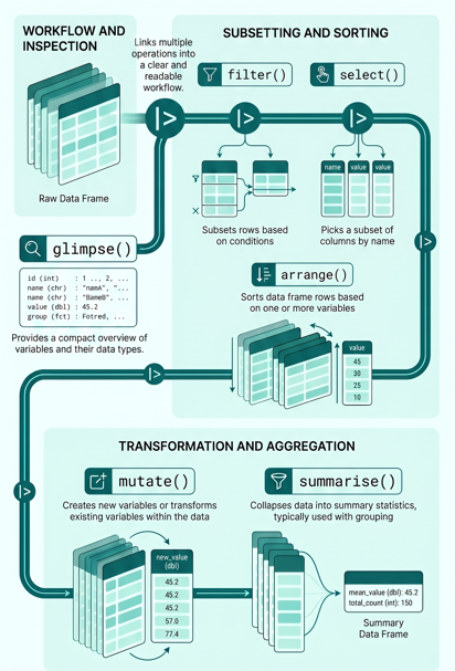
Intro to `dplyr` package

The dplyr package provides a consistent “grammar” of data manipulation with set of verbs in R.

The key operator and core verbs include:

|>: the pipe operator used to link multiple operations into a clear and readable workflow (pipeline).
select(): selects a subset of columns from a data frame.
mutate(): creates new variables or transforms existing variables.
filter(): subsets rows based on logical conditions.
arrange(): sorts rows based on one or more variables.
summarise() / summarize(): collapses data into summary statistics, often used with group_by().

The structure and content of a dataset can be quickly explored using the glimpse() function from the dplyr package, which provides a compact overview of variables and their types.

The Pipe Operator `|>`

Passes data left → right, step by step - no nesting, no temp objects

Saving each step (cluttered)

step1 <- filter(malaria, age > 15)
step2 <- select(step1, sex, region, hemoglobin)

Nesting functions (hard to read)

result <- select(
  filter(malaria, age > 15),
  sex, region, hemoglobin)

Pipe operator (clean & readable)

result <- malaria |>
  filter(age > 15) |>
  select(sex, region, hemoglobin)

Read it like a sentence: “Take malaria data, then keep age > 15, then select these columns.”

Two pipe flavours

Pipe	Package needed?	When to use
`\|>`	None (R ≥ 4.1)	Default - use this
`%>%`	`dplyr` / `magrittr`	When you need the `.` placeholder

Tip

This works cleanly with %>%: malaria %>% lm(hemoglobin ~ age + sex, data = .)
This breaks with |> but limited supprot in data = _ for >4.2.

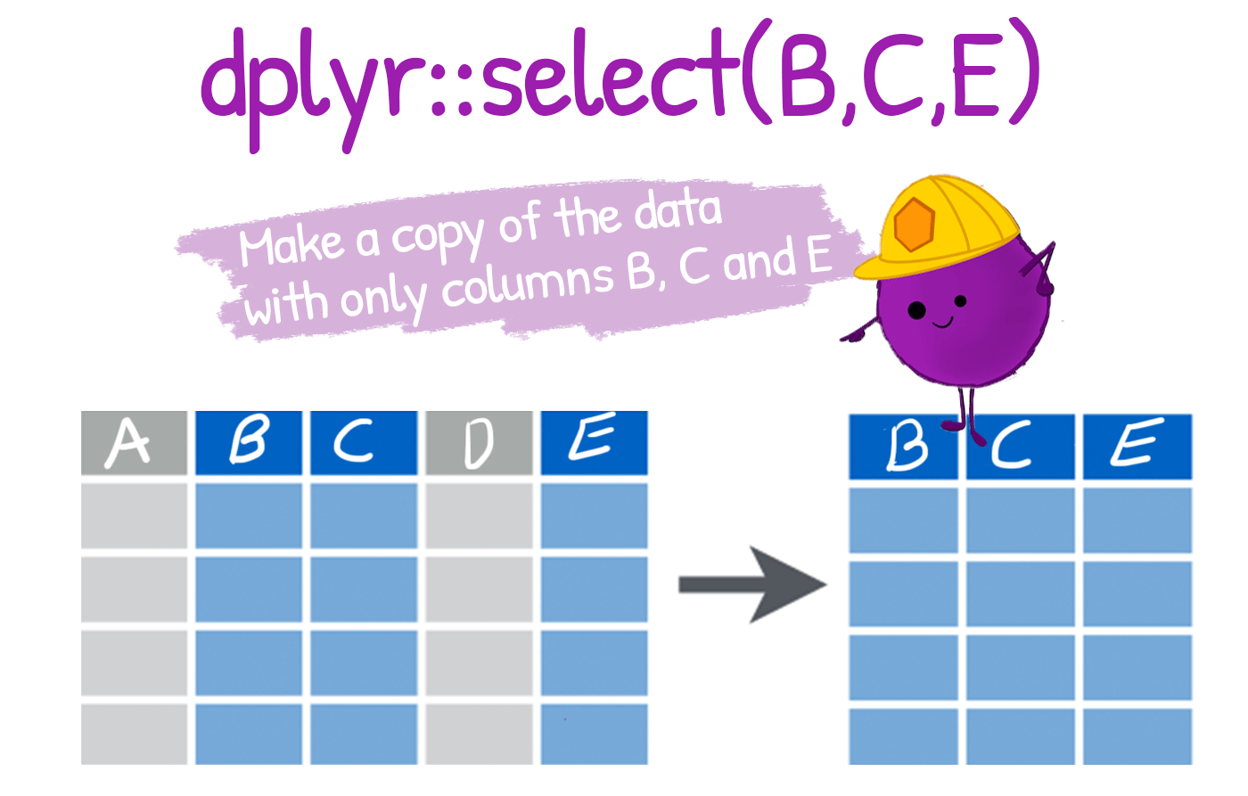
`select()`: To extract variables

Selecting variables is usually one of the first steps in data cleaning and data preparation.
It helps to simplify large datasets by keeping only the variables needed for analysis.
select() is our first verb, useful when preparing reporting datasets, indicator tables, or survey analysis datasets.
It improves workflow efficiency by reducing unnecessary columns before further transformation or analysis.

It supports flexible selection using variable names, ranges, or helper functions (e.g., starts_with(), contains()).

dplyr::select() lets us pick which columns (variables) to keep or drop. In survey work this is the first cleaning step: from dozens of collected fields, keep only the ones an analysis needs.

We can select a column by name:

Code

malaria |> select(age) |> 
  head()

# A tibble: 6 × 1
    age
  <dbl>
1    27
2    25
3    16
4     9
5    49
6     9

Or we can select a column by position:

Code

malaria |> select(3) |> head()

# A tibble: 6 × 1
  region
  <chr> 
1 Amhara
2 Amhara
3 Amhara
4 Amhara
5 Amhara
6 Amhara

To select multiple variables, we separate them with commas:

Code

malaria |> 
  select(age, sex, rdt_result) |> 
  head()

# A tibble: 6 × 3
    age sex    rdt_result
  <dbl> <chr>  <chr>     
1    27 Male   Not tested
2    25 Female Not tested
3    16 Male   Not tested
4     9 Male   Not tested
5    49 Female Not tested
6     9 Female Not tested

Select the 13th and 19th columns in the malaria data frame.
For the next part of the tutorial, let’s create a smaller subset of the data, called mis.

Code

mis <- malaria |> select(age, sex, education_level, pregnancy_status,
                          fever_last_2weeks, bednet_used, rdt_result,
                          malaria_positive, hemoglobin, region)

Selecting column ranges with `:`

The : operator selects a range of consecutive variables:

Code

mis |> 
  select(age:pregnancy_status) |> 
  head(4)

# A tibble: 4 × 4
    age sex    education_level pregnancy_status
  <dbl> <chr>  <chr>           <chr>           
1    27 Male   Primary         Not applicable  
2    25 Female Secondary       Not pregnant    
3    16 Male   Higher          Not applicable  
4     9 Male   None            Not applicable

We can also specify a range with column numbers:

Code

mis |> select(1:4) |> 
  head(4)

# A tibble: 4 × 4
    age sex    education_level pregnancy_status
  <dbl> <chr>  <chr>           <chr>           
1    27 Male   Primary         Not applicable  
2    25 Female Secondary       Not pregnant    
3    16 Male   Higher          Not applicable  
4     9 Male   None            Not applicable

Excluding columns with `!`

The exclamation point negates a selection:

Code

mis |> select(!age) |> head(3)

# A tibble: 3 × 9
  sex    education_level pregnancy_status fever_last_2weeks bednet_used
  <chr>  <chr>           <chr>            <chr>             <chr>      
1 Male   Primary         Not applicable   No                Yes        
2 Female Secondary       Not pregnant     No                No         
3 Male   Higher          Not applicable   No                No         
# ℹ 4 more variables: rdt_result <chr>, malaria_positive <chr>,
#   hemoglobin <dbl>, region <chr>

To drop consecutive columns:!age:pregnancy_status:

Code

mis |> 
  select(!age:pregnancy_status) |> head(3)

# A tibble: 3 × 6
  fever_last_2weeks bednet_used rdt_result malaria_positive hemoglobin region
  <chr>             <chr>       <chr>      <chr>                 <dbl> <chr> 
1 No                Yes         Not tested <NA>                   13.4 Amhara
2 No                No          Not tested <NA>                   11.5 Amhara
3 No                No          Not tested <NA>                   11.4 Amhara

To drop several non-consecutive columns, place them inside !c():

Code

mis |> select(!c(age, sex, rdt_result)) |> head()

Helper functions for `select()`

dplyr has a number of helper functions to make selecting easier by using patterns from the column names. Let’s take a look at some of these.
starts_with() and ends_with(): these two helpers work exactly as their names suggest!

Code

malaria |> 
  select(starts_with("bednet_")) |> 
  head(4)

# A tibble: 4 × 3
  bednet_owned bednet_used bednet_condition
  <chr>        <chr>       <chr>           
1 Yes          Yes         Worn            
2 No           No          No net          
3 No           No          No net          
4 No           No          No net

Code

malaria |>
  select(ends_with("_result")) |> 
  head(4)

# A tibble: 4 × 1
  rdt_result
  <chr>     
1 Not tested
2 Not tested
3 Not tested
4 Not tested

`contains()`

contains() helps select columns that contain a certain string:

Code

malaria |> select(contains("malaria")) # Columns that contain the string "malaria"

`everything()`

Another helper function, everything(), useful for establishing the order of columns.
- eg, to bring the rdt_result column to the start of the mis data frame, we could type out all the column names manually or using everything() function:

Code

mis |> 
  select(rdt_result, everything())

Code

mis |> 
  select(rdt_result, age, sex, education_level, 
         pregnancy_status, fever_last_2weeks, 
         bednet_used, malaria_positive, region,
         hemoglobin)

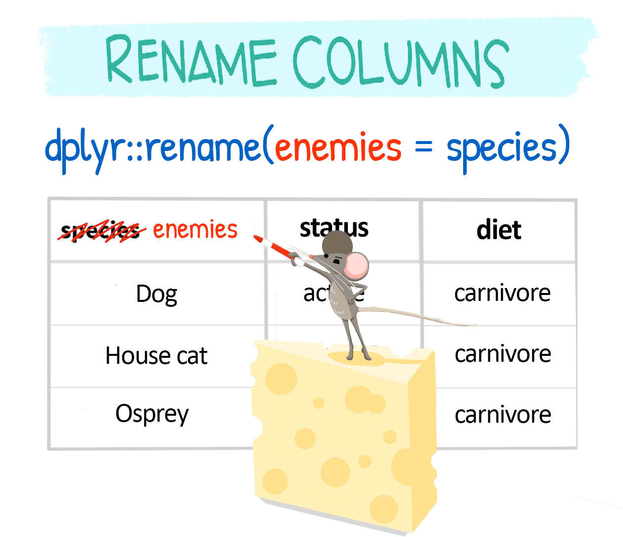
Change column names with `rename()`

dplyr::rename() is used to change column names:

rename() changes chosen columns (new = old):

Code

malaria |>
  rename(patient_age = age, 
         patient_sex = sex)

Rename within `select()`

You can also rename columns while selecting them:

Code

malaria |>
  select(patient_age = age, patient_sex = sex)

Advance `select()` functions

You can also select columns based on their data type using where() using select(where(is.numeric)).
The common type tests are: is.character, is.double, is.factor, is.integer, is.logical, is.numeric.
rename_with() applies a function to many names at once, rename_with(toupper)

Code

malaria |> rename_with(toupper) |> 
  select(where(is.numeric))

Also the following are other important function
- _all() if you want to apply the function to all columns
- _at() if you want to apply the function to specific columns (specify them with vars())
- _if() if you want to apply the function to columns of a certain characteristic (e.g. data type)
- _with() if you want to apply the function to columns and include another function within it

Note

These variants are quite flexible, and keep changing for individual functions (eg,. rename_with(), rename_all(), rename_at(), rename_if()).

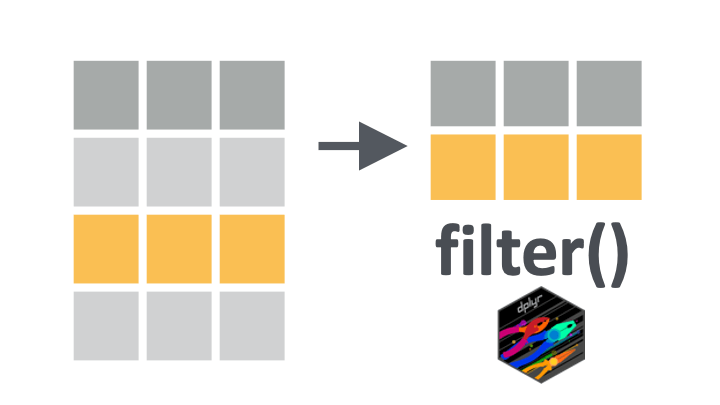
`filter()`

Dropping abnormal data entries or keeping subsets of your data points is another essential aspect of data wrangling.

filter(dataframe, logical statement 1, logical statement 2, ...)
We use filter() to keep rows that satisfy a set of conditions.
If we want to keep just the male records, we run:

Code

mis |> filter(sex == "Male") |> 
  nrow()
#to get the number of rows fulfilling a condition.

Note the use of the double equal sign == rather than the single equal sign =.

Fig: the filter() verb.

So the code mis |> filter(sex == "Male") will keep all rows.

Relational operators

The == operator introduced above is an example of a “relational” operator, as it tests the relation between two values. Here is a list of some of these operators:

Operator	is TRUE if
A < B	A is less than B
A <= B	A is less than or equal to B
A > B	A is greater than B
A >= B	A is greater than or equal to B
A == B	A is equal to B
A != B	A is not equal to B
A %in% B	A is an element of B

Let’s see how to use these within filter():

Code

mis |> filter(sex != "Male") ## keep rows where `sex` is not "Male"
mis |> filter(age < 5) ## keep children under 5 (a key malaria risk group)
mis |> filter(age >= 65) ## keep respondents aged at least 65

### keep respondents whose education is "Primary" or "Secondary"
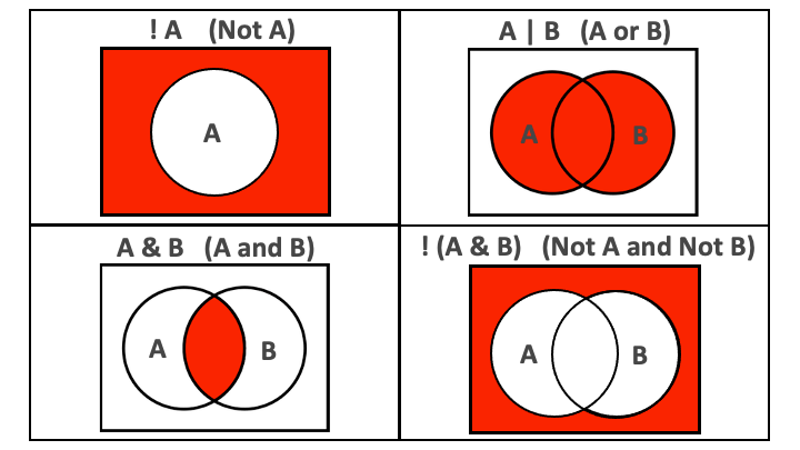
mis |> filter(education_level %in% c("Primary", "Secondary"))

Combining conditions with `&` and `|`

We can pass multiple conditions to a single filter() statement separated by commas:

keep women who are pregnant and did not sleep under a bednet

Code

mis |> 
  filter(pregnancy_status == "Pregnant", 
         bednet_used == "No")

same result as before, but & is more explicit

Code

mis |> 
  filter(pregnancy_status == "Pregnant" & 
           bednet_used == "No")

When multiple conditions are separated by a comma, they are implicitly combined with an and (&).
It is best to replace the comma with & to make this more explicit.

Side Note

Don’t confuse:

the “,” in listing several conditions in filter filter(A,B) i.e. filter based on condition A and (&) condition B
the “,” in lists c(A,B) which is listing different components of the list (and has nothing to do with the & operator)

If we want to combine conditions with an or, we use the vertical bar symbol, |.

Code

### respondents who are pregnant OR who did not use a bednet
mis |> filter(pregnancy_status == "Pregnant" | bednet_used == "No")

Negating conditions with `!`

To negate conditions, we wrap them in !().
Below, we drop respondents who are children (less than 5 years) or who are anemic (hemoglobin below 11 g/dL):

Code

### drop respondents < 5 years OR hemoglobin < 11
mis |> filter(!(age < 5 | hemoglobin < 11))

The ! operator is also used to negate %in% since R does not have an operator for NOT in.

Code

### drop respondents whose education is NOT "Primary" or "Secondary"
mis |> filter(!(education_level %in% c("Primary", "Secondary")))

Key Point

It is easier to read filter() statements as keep statements, to avoid confusion over whether we are filtering in or filtering out!
So the code below would read: “keep respondents who are under 5 or who are anemic (hemoglobin under 11)”.

Code

mis |> filter(age < 5 | hemoglobin < 11)

And when we wrap conditions in !(), we can then read filter() statements as drop statements.

So the code below would read: “drop respondents who are under 5 or who are anemic (hemoglobin under 11)”.

Code

mis |> filter(!(age < 5 | hemoglobin < 11))

Filtering on a numeric range with `between()`

For a numeric range you could write two conditions, but between() is shorter and clearer. Here we keep individuals whose hemoglobin sits in the mild-anemia band (11 to 13 g/dL):

Code

malaria |>
  select(individual_id, sex, hemoglobin) |>
  filter(between(hemoglobin, 11, 13)) |> head()

# A tibble: 6 × 3
  individual_id sex    hemoglobin
  <chr>         <chr>       <dbl>
1 HH-00001-02   Female       11.5
2 HH-00001-03   Male         11.4
3 HH-00001-04   Male         11.1
4 HH-00001-05   Female       12.4
5 HH-00001-06   Female       12.6
6 HH-00002-01   Male         11.2

Key Point

filter(between(hemoglobin, 11, 13)) is equivalent to filter(hemoglobin >= 11, hemoglobin <= 13).

Filtering across multiple columns with `if_any()` / `if_all()`

To apply one condition to several columns at once, use if_any() (any column meets it, like OR) or if_all() (every column meets it, like AND). These replace the older filter_all(), filter_at(), and filter_if() helpers.

Code

# households missing protection on ANY bednet measure
malaria |>
  filter(if_any(c(bednet_owned, bednet_used), ~ .x == "No"))

Code

# people who BOTH had a fever AND were tested
malaria |>
  filter(if_all(c(fever_last_2weeks, malaria_tested), ~ .x == "Yes"))

Tip

if_any()/if_all() accept the same column selectors as select() (names, starts_with(), where(is.numeric)), so one pattern covers many filtering needs.

Filltering Missing values

The relational operators introduced so far do not work with NA.

The special function is.na() is therefore necessary:

Code

### keep rows where `malaria_positive` is NA (people not tested)
mis_mini |> filter(is.na(malaria_positive))

This function can be negated with !:

Code

### drop rows where `malaria_positive` is NA (keep only those tested)
mis_mini |> filter(!is.na(malaria_positive))

Creating new variables with `mutate()`

mutate() adds new columns while keeping the existing ones.
In survey work this is how we build indicators: turning raw fields into the variables an analysis actually needs.
- mutate() adds new variables, keeping the old ones.
- across() applies the same transformation to several columns at once (the modern replacement for mutate_all(), mutate_at(), and mutate_if()).

Code

library(dplyr)
ex <- malaria |>
   mutate(anemic = hemoglobin < 11,            # new TRUE/FALSE indicator
              far_from_clinic = distance_health_facility > 10)

Transform many columns at once with `across()`

across() inside mutate() applies one function to several columns in a single step.
It is the recommended replacement for the older mutate_all(), mutate_at(), and mutate_if() helpers.

Code

ex_num <- malaria |> 
  mutate(across(c(hemoglobin, distance_health_facility), round))
head(ex_num)

# A tibble: 6 × 28
  individual_id household_id region zone   woreda    kebele       household_size
  <chr>         <chr>        <chr>  <chr>  <chr>     <chr>                 <dbl>
1 HH-00001-01   HH-00001     Amhara AMH-Z5 AMH-Z5-W2 AMH-Z5-W2-K…              8
2 HH-00001-02   HH-00001     Amhara AMH-Z5 AMH-Z5-W2 AMH-Z5-W2-K…              8
3 HH-00001-03   HH-00001     Amhara AMH-Z5 AMH-Z5-W2 AMH-Z5-W2-K…              8
4 HH-00001-04   HH-00001     Amhara AMH-Z5 AMH-Z5-W2 AMH-Z5-W2-K…              8
5 HH-00001-05   HH-00001     Amhara AMH-Z5 AMH-Z5-W2 AMH-Z5-W2-K…              8
6 HH-00001-06   HH-00001     Amhara AMH-Z5 AMH-Z5-W2 AMH-Z5-W2-K…              8
# ℹ 21 more variables: wealth_quintile <chr>, distance_health_facility <dbl>,
#   altitude <dbl>, rainfall_mm <dbl>, irs_received <chr>, age <dbl>,
#   sex <chr>, pregnancy_status <chr>, education_level <chr>,
#   fever_last_2weeks <chr>, malaria_tested <chr>, rdt_result <chr>,
#   malaria_positive <chr>, treatment_received <chr>, bednet_owned <chr>,
#   bednet_used <chr>, bednet_condition <chr>, hemoglobin <dbl>,
#   anemia_status <chr>, bmi <dbl>, nutritional_status <chr>

Code

# round every numeric column (selection by type)
ex_num |> mutate(across(where(is.numeric), round, digits = 2))

# A tibble: 26,264 × 28
   individual_id household_id region         zone   woreda kebele household_size
   <chr>         <chr>        <chr>          <chr>  <chr>  <chr>           <dbl>
 1 HH-00001-01   HH-00001     Amhara         AMH-Z5 AMH-Z… AMH-Z…              8
 2 HH-00001-02   HH-00001     Amhara         AMH-Z5 AMH-Z… AMH-Z…              8
 3 HH-00001-03   HH-00001     Amhara         AMH-Z5 AMH-Z… AMH-Z…              8
 4 HH-00001-04   HH-00001     Amhara         AMH-Z5 AMH-Z… AMH-Z…              8
 5 HH-00001-05   HH-00001     Amhara         AMH-Z5 AMH-Z… AMH-Z…              8
 6 HH-00001-06   HH-00001     Amhara         AMH-Z5 AMH-Z… AMH-Z…              8
 7 HH-00001-07   HH-00001     Amhara         AMH-Z5 AMH-Z… AMH-Z…              8
 8 HH-00001-08   HH-00001     Amhara         AMH-Z5 AMH-Z… AMH-Z…              8
 9 HH-00002-01   HH-00002     South Ethiopia SOU-Z5 SOU-Z… SOU-Z…              7
10 HH-00002-02   HH-00002     South Ethiopia SOU-Z5 SOU-Z… SOU-Z…              7
# ℹ 26,254 more rows
# ℹ 21 more variables: wealth_quintile <chr>, distance_health_facility <dbl>,
#   altitude <dbl>, rainfall_mm <dbl>, irs_received <chr>, age <dbl>,
#   sex <chr>, pregnancy_status <chr>, education_level <chr>,
#   fever_last_2weeks <chr>, malaria_tested <chr>, rdt_result <chr>,
#   malaria_positive <chr>, treatment_received <chr>, bednet_owned <chr>,
#   bednet_used <chr>, bednet_condition <chr>, hemoglobin <dbl>, …

Tip

across(c(...)) selects columns by name; across(where(is.numeric)) selects by type. The same idea works inside summarise().

Sort rows with `arrange()`

arrange() re-orders rows, ascending by default. Wrap a variable in desc() for descending order: arrange(data, var1, desc(var2), ...).
Here we sort individuals by region, then from the most anemic downward, to surface the people who may need follow-up first:

Code

malaria |>
  select(individual_id, region, hemoglobin) |>
  arrange(region, desc(hemoglobin)) |> head()

# A tibble: 6 × 3
  individual_id region hemoglobin
  <chr>         <chr>       <dbl>
1 HH-00657-06   Afar         18  
2 HH-02676-01   Afar         18  
3 HH-02840-03   Afar         17.7
4 HH-04089-03   Afar         17.4
5 HH-04430-05   Afar         17.4
6 HH-00534-02   Afar         17.3

Tip

Try arrange(hemoglobin) (ascending) versus arrange(desc(hemoglobin)) and watch which rows rise to the top.

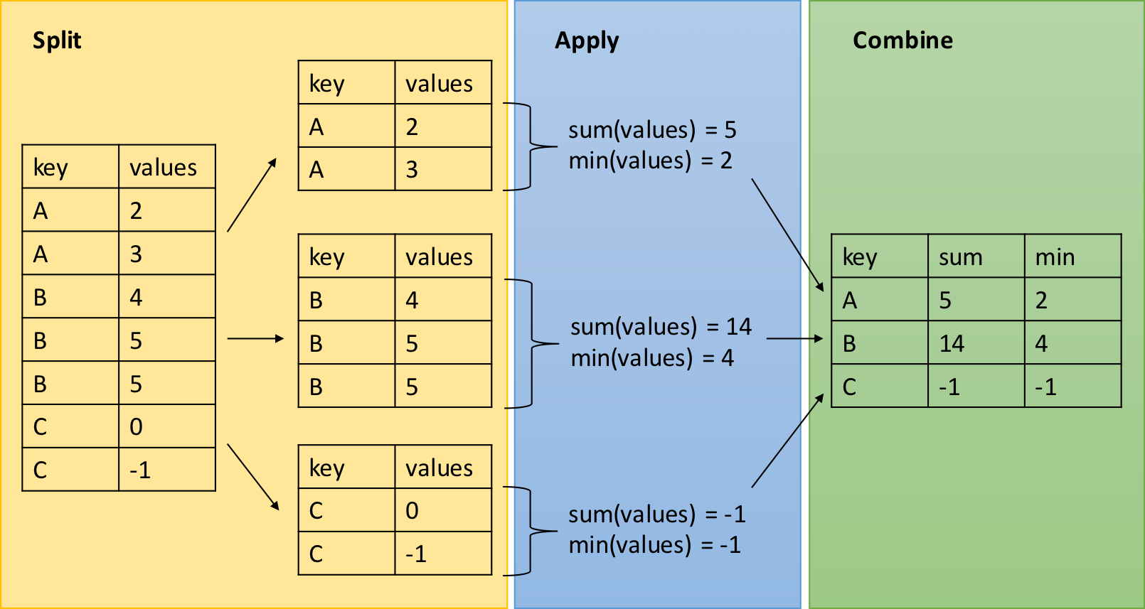
`group_by()` and `summarise()`

The dplyr verbs become especially powerful when they are are combined using the pipe operator |>.

The following dplyr functions allow us to split our data frame into groups on which we can perform operations individually
group_by(): group data frame by a factor for downstream operations (usually summarise)
summarise(): summarise values in a data frame or in groups within the data frame with aggregation functions (e.g. min(), max(), mean(), etc…)

dplyr - Split-Apply-Combine

The group_by function is key to the Split-Apply-Combine strategy

Test positivity by region (the key MIS indicator)

The most important malaria survey number is the test positivity rate: of the people who were tested, what share were positive. group_by() plus summarise() gives it to us for every region in one step.

Code

positivity <- malaria |> group_by(region) |>
  summarise(
    n_tested = sum(malaria_tested == "Yes"),
    n_positive = sum(malaria_positive == "Yes", na.rm = TRUE),
    positivity_pct = round(100*n_positive / n_tested, 1)) |> arrange(desc(positivity_pct))
positivity

# A tibble: 8 × 4
  region            n_tested n_positive positivity_pct
  <chr>                <int>      <int>          <dbl>
1 Gambella               686        358           52.2
2 Benishangul Gumuz      655        233           35.6
3 Afar                   829        181           21.8
4 Somali                 606        112           18.5
5 South Ethiopia         411         13            3.2
6 Oromia                 842         24            2.9
7 Sidama                 230          4            1.7
8 Amhara                 655          9            1.4

How to read this

Lowland regions (Gambella, Benishangul Gumuz) sit far above the highlands (Amhara, Sidama). This pattern, not a single national average, is what guides where to send nets and spraying.

The same numbers, as a picture

A summary table becomes far more persuasive as a chart. The positivity gradient across regions is obvious at a glance:

Code

library(ggplot2)
positivity |>
  ggplot(aes(x = reorder(region, positivity_pct), 
             y = positivity_pct)) +
  geom_col(fill = "#047B77") +
  geom_text(aes(label = paste0(positivity_pct, "%")), 
            hjust = -0.15, size = 3.5) +
  coord_flip() +
  labs(x = NULL, y = "Test positivity (%)",
       title = "Malaria test positivity by region") +
  theme_minimal(base_size = 13)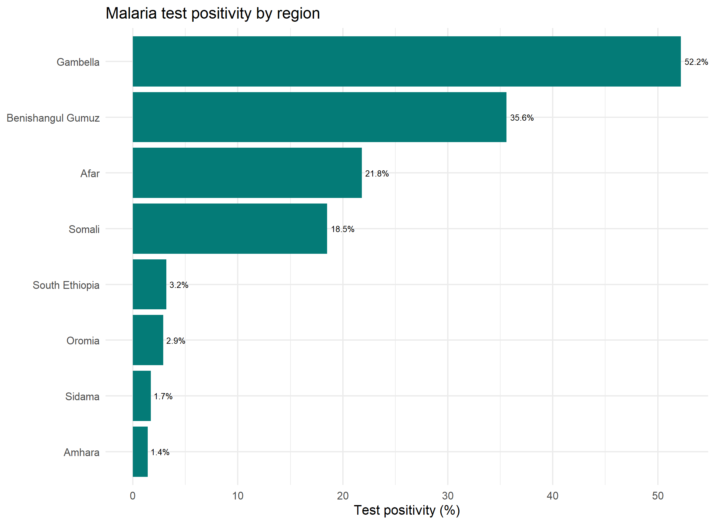

Summarising many columns with `across()`

To compute the same statistic over several columns, use across() inside summarise().
This is the modern replacement for summarize_all(), summarize_at(), and summarize_if().

Code

malaria |>
  group_by(region) |>
  summarise(across(c(hemoglobin, distance_health_facility, altitude),
                   ~ round(mean(.x, na.rm = TRUE), 1)))

# A tibble: 8 × 4
  region            hemoglobin distance_health_facility altitude
  <chr>                  <dbl>                    <dbl>    <dbl>
1 Afar                    12.8                      7.7     552.
2 Amhara                  12.9                      7.8    2295.
3 Benishangul Gumuz       12.7                      8.1     882.
4 Gambella                12.5                      7.1     508.
5 Oromia                  12.9                      7.7    2011.
6 Sidama                  12.9                      8      2132.
7 Somali                  12.8                      7.7     656.
8 South Ethiopia          12.9                      8      1696.

Select columns by name (c(...)), by type (where(is.numeric)), or by pattern (starts_with("bednet")), exactly as in select().

Recoding messy field entries

A common headache: enumerators record the same answer many ways.
Here, an RDT result column collected by different field teams:

Code

library(dplyr)
raw_malaria <- tibble(
  individual_id = sprintf("P-%02d", 1:12),
  region = c("Amhara","amhara","Oromia","oromia","Somali","somali",
             "Gambella","gambella","Afar","afar","Sidama","sidama"),
  result = c("Pos","positive","P","Neg","negative","N",
             "POS","Positive","Negative","neg","pos","NEG"))
#write.csv(raw_malaria, "raw_malaria.csv")

Twelve rows, but the result is written eight different ways.
We need to standardize before any analysis.

`recode()`: map old values to new

recode() inside mutate() rewrites specific values.
List each old value and what it should become:

Code

raw_malaria |>
  mutate(result = recode(result,
           Pos = "Positive", P = "Positive", POS = "Positive",
           pos = "Positive", positive = "Positive",
           Neg = "Negative", N = "Negative", NEG = "Negative",
           neg = "Negative", negative = "Negative")) |>
  count(result)

# A tibble: 2 × 2
  result       n
  <chr>    <int>
1 Negative     6
2 Positive     6

Warning

recode() is fine for a short, fixed list, but it gets unwieldy fast. For anything with rules or ranges, reach for case_when().

`case_when()`: rule-based recoding

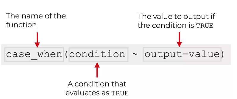
case_when() checks conditions top to bottom. Any value not matched becomes NA unless you add a final TRUE ~ ... catch-all.

Code

raw_malaria |>
  mutate(result_clean = case_when(
    result %in% c("Pos","P","POS","pos","positive","Positive") ~ "Positive",
    result %in% c("Neg","N","NEG","neg","negative","Negative") ~ "Negative",
    TRUE ~ "Unknown")) |>               # catch-all keeps the rest visible
  count(result_clean)

# A tibble: 2 × 2
  result_clean     n
  <chr>        <int>
1 Negative         6
2 Positive         6

Two-level indicators with `if_else()`

To turn a numeric variable into a yes/no category, if_else() is the cleanest tool.
Here we flag anemia from hemoglobin:

Code

malaria |>
  mutate(anemia_flag = if_else(hemoglobin < 11, "Anemic", "Not anemic")) |>
  count(anemia_flag)

# A tibble: 2 × 2
  anemia_flag     n
  <chr>       <int>
1 Anemic       3478
2 Not anemic  22786

Use of `naniar` and `janitor` packages for data cleaning

`naniar`

used to work with missing data
Sometimes you need to look at lots of data though… the naniar package is a good option.
The pct_complete() function shows the percentage that is complete for a given data object, (vector or data frame).

Code

#install.packages("naniar")
library(naniar)
pct_complete(malaria)   # % of all cells that are non-missing

[1] 95.18638

Code

# malaria_positive is missing for everyone not tested
malaria |> select(malaria_positive) |>
  pct_complete()

[1] 18.71002

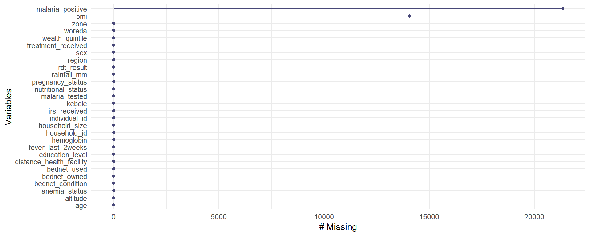
`naniar` plots

The gg_miss_var() function creates a nice plot about the number of missing values for each variable, (need a data frame).

Code

malaria |>
   gg_miss_var()

To remove rows with `NA` values for a variable use `drop_na()`

A function from the tidyr package. (Need a data frame to start!)
Don’t do this unless you have thought about if dropping NA values makes sense based on knowing what these values mean in your data.

Code

library(tidyr)
malaria |> drop_na(nets_owned)

Code

malaria |> drop_na()

Change a value to be `NA`

The na_if() function of dplyr is useful when a sentinel value was used for “not recorded”. Here a 0 in nets_owned really meant missing, so we convert it to NA.

Code

malaria |>
  mutate(nets_owned = na_if(nets_owned, 0))

`janitor`

Used for data cleaning, which is one of the most essential parts of analysis: turning messy field data into something reliable you can analyze in R.
Common tasks:
- fix ugly column names,
- drop blank rows or columns,
- remove duplicate rows, and
- check consistency with frequency tables.

The janitor package handles all of these.

Some functions of `janitor`

clean_names(): standardizes column names:

lower case, separated by underscores, no spaces or special characters. This is almost always the first step after importing a survey export.
Here is a small, messy survey extract: ugly column names, an empty column, a constant column, and a duplicated row.

Code

library(janitor)
dirty <- tibble(
  `Household ID`     = c("HH-01","HH-02","HH-02","HH-03"),
  `Region `          = c("Amhara","Oromia","Oromia","Somali"),
  `RDT Result (+/-)` = c("Positive","Negative","Negative","Positive"),
  notes              = NA,        # completely empty column
  survey_year        = 2024)      # constant column
clean <- clean_names(dirty)       # tidy the column names
clean

# A tibble: 4 × 5
  household_id region rdt_result notes survey_year
  <chr>        <chr>  <chr>      <lgl>       <dbl>
1 HH-01        Amhara Positive   NA           2024
2 HH-02        Oromia Negative   NA           2024
3 HH-02        Oromia Negative   NA           2024
4 HH-03        Somali Positive   NA           2024

remove_empty() & remove_constant()

remove_empty() drops fully blank rows or columns; remove_constant() drops columns that never vary.
Together they strip out the notes and survey_year junk:

Code

tidy_extract <- clean |>
  remove_empty(which = c("rows", "cols")) |>
  remove_constant()
tidy_extract

# A tibble: 4 × 3
  household_id region rdt_result
  <chr>        <chr>  <chr>     
1 HH-01        Amhara Positive  
2 HH-02        Oromia Negative  
3 HH-02        Oromia Negative  
4 HH-03        Somali Positive

get_dupes(): examine duplicate rows

get_dupes() returns the duplicated rows with a dupe_count column, so you can decide whether a repeat is a true duplicate or two real people. HH-02 appears twice:

Code

clean |> get_dupes(household_id)

# A tibble: 2 × 6
  household_id dupe_count region rdt_result notes survey_year
  <chr>             <int> <chr>  <chr>      <lgl>       <dbl>
1 HH-02                 2 Oromia Negative   NA           2024
2 HH-02                 2 Oromia Negative   NA           2024

distinct() from dplyr then keeps one copy of each unique row:

Code

clean |> distinct(household_id, .keep_all = TRUE)

# A tibble: 3 × 5
  household_id region rdt_result notes survey_year
  <chr>        <chr>  <chr>      <lgl>       <dbl>
1 HH-01        Amhara Positive   NA           2024
2 HH-02        Oromia Negative   NA           2024
3 HH-03        Somali Positive   NA           2024

Excercises

Keep only individual_id, region, age, and rdt_result.
Select all the bednet variables using a helper.
Keep every column except zone, woreda, and kebele.
Select only the numeric columns.
Keep children under 5 years old.
Keep individuals who were tested and had a positive RDT.
Keep people in Gambella or Benishangul Gumuz whose hemoglobin is below 11.
Keep rows where the person was not tested.
How many pregnant women did not sleep under a bednet? (combine filter() with nrow()).
Create far_from_clinic = "Yes" when distance_health_facility > 10, else "No" (use if_else()).
Create an age_group column with case_when() and recode(): "Under 5", "5-14", "15-49", "50+".
For each region, compute the number tested and the test positivity rate (% positive among tested). Sort from highest positivity.
Compare positivity for net users vs non-users (group by bednet_used, among the tested).

Data Manipulation and Cleaning using dplyr() package

What is Tidyverse?

install.packages(“tidyverse”)

read() and haven() packages

The Ethiopian malaria survey dataset

Load the data

The survey at a glance

Intro to dplyr package

The Pipe Operator |>

Two pipe flavours

select(): To extract variables

Selecting column ranges with :

Excluding columns with !

Helper functions for select()

contains()

everything()

Change column names with rename()

Rename within select()

Advance select() functions

filter()

Relational operators

Combining conditions with & and |

Negating conditions with !

Filtering on a numeric range with between()

Filtering across multiple columns with if_any() / if_all()

Filltering Missing values

Creating new variables with mutate()

Transform many columns at once with across()

Sort rows with arrange()

group_by() and summarise()

Test positivity by region (the key MIS indicator)

The same numbers, as a picture

Summarising many columns with across()

Recoding messy field entries

recode(): map old values to new

case_when(): rule-based recoding

Two-level indicators with if_else()

Use of naniar and janitor packages for data cleaning

naniar

naniar plots

To remove rows with NA values for a variable use drop_na()

Change a value to be NA

janitor

Some functions of janitor

Excercises

Thank You!

Data Manipulation and Cleaning using `dplyr()` package

`read()` and `haven()` packages

Intro to `dplyr` package

The Pipe Operator `|>`

`select()`: To extract variables

Selecting column ranges with `:`

Excluding columns with `!`

Helper functions for `select()`

`contains()`

`everything()`

Change column names with `rename()`

Rename within `select()`

Advance `select()` functions

`filter()`

Combining conditions with `&` and `|`

Negating conditions with `!`

Filtering on a numeric range with `between()`

Filtering across multiple columns with `if_any()` / `if_all()`

Creating new variables with `mutate()`

Transform many columns at once with `across()`

Sort rows with `arrange()`

`group_by()` and `summarise()`

Summarising many columns with `across()`

`recode()`: map old values to new

`case_when()`: rule-based recoding

Two-level indicators with `if_else()`

Use of `naniar` and `janitor` packages for data cleaning

`naniar`

`naniar` plots

To remove rows with `NA` values for a variable use `drop_na()`

Change a value to be `NA`

`janitor`

Some functions of `janitor`