Spatial Data Analysis Training

Yebelay Berehan

National Data Management Center for Health at EPHI and AAU Department of Statistics

December 25-29, 2024

Outlines ….. (1)

Source, Format, and Types of Spatial Data

What is GIS? What is spatial data and why should we use it?
Types of spatial data
Formats of Spatial Data
Sources of Spatial Data/ Exploring spatial data

Basic R Packages for Spatial Data Management and Modelling

Installing basic packages
Data Management Packages
Data Visualization and Mapping Packages
Modelling Packages

Outlines ….. (2)

Overview of spatial and non-spatial data analysis framework
Spatial Exploratory Data Analysis
- Spatial weight construction
- Case studies and practical session
Investigating spatial dependence
Spatial modeling framework
- Areal Data modeling
Geostatistical Modeling

Source, Format, and Types of Spatial Data

What is GIS? What is spatial data and why should we use it?

GIS (Geographical Information Systems):
- A system designed to capture, store, manipulate, analyze, manage, and visualize spatial or geographic data.
- Integrates data from multiple sources to provide insights into spatial patterns and relationships.
Spatial data, also known as geospatial data, refers to information that identifies the geographic location and characteristics of natural or constructed features and boundaries on the Earth.
This data is often represented in terms of Cartesian coordinates (x,y) for two-dimensional maps, but may also include altitude (z) for a three-dimensional representation.
Spatial data is essential for analyzing relationships within a geographical context.
- It is widely used in health helps map disease spread, identify hotspots, allocate resources, and monitor environmental impacts on health, and urban planning.

Spatial Data can be collected in either
- Satellite Imagery: Captured by remote sensing satellites, these images can provide data on land cover, vegetation, weather patterns, and more.
- GPS Surveys: Use Global Positioning System technology to collect precise location data for mapping and navigation purposes.
- Traditional Surveying Methods: Involve measuring angles, distances, and elevations to map out areas accurately, often using tools like theodolites and total stations.

Spatial Data Formats

Let us see a basic way to represent the spatial data.
But there is a variety of data formats to represent the data to suit different applications.
In most cases, spatial data formats are an extension of existing data formats.

Spatial Data Formats Categorized by Type

Spatial Data Formats Categorized by Type

Type	Spatial Data Formats
Text Files	CSV: Enhanced with spatial attributes (e.g., coordinates). GeoJSON: Representing points, lines, polygons, and metadata. GML: for representing geographic features and metadata. KML: used for Google Earth and online maps.
Binary/Compressed	Shapefile: A multi-file format storing vector data (geometry and attributes). GeoPDF: Geospatially enabled PDF with embedded layers and coordinate data. Geopackage: supporting both vector and raster data. PBF: Binary format for OpenStreetMap data, efficient for large datasets.
Images	GeoTIFF: metadata for raster data. JPEG2000: Compressed image format for multi-resolution datasets. ECW: Compressed raster format optimized for large imagery datasets.
Databases	Spatialite: supporting spatial data and functions. PostGIS: enabling advanced spatial queries and storage. Oracle Spatial: supporting 3D and network data. ArcGIS Geodatabase: spatial database format for managing geographic datasets.

Spatial Data Types

Spatial Data can be broadly categorized into 2 types - Vector and Raster.
- But what is the difference between raster and vector data?
- *When should we use raster and when should we use vector features?_

Vector Data: Overview

Vectors are representations of spatial data using points, lines, and polygons.
- They represent real-world features at varying levels of detail, depending on the map scale.
Unlike rasters, vectors are not made up of grids or pixels. Instead, they consist of:
- Vertices: Specific coordinate points.
- Paths: Lines connecting the vertices.
Points: are individual XY coordinates, typically latitude and longitude, with a spatial reference frame.
- They are used to represent features too small to be displayed as polygons.
  - Example: Cities shown as points on a global map.
- They are simple, precise locations, and they are efficient for small-scale maps.

Lines connect multiple vertices using paths, forming linear features (e.g., Rivers, roads, and pipelines).
Polygons are formed by connecting vertices in a closed path (e.g., Building footprints, agricultural fields).
- Used to represent areas with measurable attributes (e.g., square footage, acreage).
- First and last coordinates of a polygon are the same to close the shape.
Vector data are high accuracy and aesthetically pleasing graphics.
- Not dependent on grid size and they are ideal for network analysis.
But processing can be intensive due to complex topology rules.

Raster Data: Overview

Raster data is a grid of pixels (or grid cells) where each cell represents a value. Values can represent various attributes like:
- Colors (e.g., satellite images), Elevation (e.g., digital elevation models) and Continuous phenomena (e.g., temperature, rainfall).
Raster data can be either discrete or continuous.
- Discrete Rasters: Represent distinct classes or categories (eg.: Land cover types (e.g., urban = 1, forest = 2).
- Consist of integers to define clear boundaries.
- Continuous Rasters: Represent data that changes gradually (eg.: Elevation, temperature).
  - Derived from a fixed reference point (e.g., sea level).
Raster data are easy to understand and perform map algebra operations.
- They are inefficient for linear or network data, large file sizes with increased resolution.

Summary of Vector vs Raster datas

Type Vector Data	Sub type Points: Represents features with a single coordinate pair (x, y). Ex.: Locations of ATMs, tree Lines: Represents linear features as ordered sequences of points. Ex.: Roads, rivers, utility lines Polygons (areas): Represents areas enclosed by closed loops of lines. Ex.: Buildings, lakes, zones

Raster Data	Grids: Represents continuous data across a surface. Satellite images, digital elevation models (DEMs) Pixels: Smallest units in a raster dataset, each with a specific value. Values representing color, temperature,
Additional information (Attribute data):	Describing the characteristics of spatial features. For example in Vector data: hospital: have hospiatl name, id, location, patient count, department Roads:have road type, traffic volume, maintenance status. In Raster Data: Each pixel can have multiple attributes, such as vegetation type or pollution levels.

What are the most common Vector data formats?

Commonly used Vector data Formats:

File Type	Description and Extension
Shapefile	The most common geospatial file and the three mandatory files to make up a shapefile are. SHP is the feature geometry. SHX is the shape index position. DBF is the attribute data. Other optional files include these files, but they are not completely necessary. PRJ(projection system), XML (associated metadata), SBN(spatial index for optimizing queries), SBX (optimizes loading times).
GeoJSON	Geographic java sript Object Notation (.GeoJSON) encodes geographic features (points, lines, polygons) in JSON format. widely used format for online web mapping.
GML(Geography Markup Language)	allows for the use of geographic coordinates extension of XML. stores geographic entities (features) in the form of text. Each feature includes properties, geometry, and a spatial reference system.

What are the most common Raster data formats?

Commonly used Raster data Formats:

File Type	Description
GeoTIFF (`.tif`, `.tiff`)	A widely used raster format that includes spatial metadata, allowing georeferencing of images.
JPEG2000 (`.jp2`, `.j2k`)	An advanced image compression format supports geospatial metadata for GIS applications.
Erdas Imagine (`.img`)	Used for remote sensing data in Erdas Imagine software.
ECW (Enhanced Compressed Wavelet) `.ecw`	A highly compressed raster format optimized for large satellite imagery and aerial photos.

What are the components of spatial data

Geometry: Refers to the coordinates that define the shape of an object.
- Coordinates: These can be in different coordinate systems, such as geographic (latitude) and longitude) or projected systems.
- Types of Geometries: Common types include points, lines, and polygons.
- Dimension: Geometry can also have dimensional attributes like 2D (x, y), 3D (x, y, z), or even 4D (x, y, z, time).
Topology: Defines spatial relationships like adjacency, connectivity, and containment.

Rules:
- No overlaps.
- Lines meet at nodes.
- Closed polygon boundaries.

Attribute Data: provide detailed information about spatial features.

Coordinate Reference Systems (CRS):

Geospatial data relies on CRS to define locations on the Earth’s surface.
A CRS contains both a datum and a projection.
Common CRS include WGS84 (GPS coordinates) and UTM (Universal Transverse Mercator).

Commonly Used EPSG Codes

WGS84(EPSG:4326) – World Geodetic System (created in) 1984.
- Used globally (e.g., Google Earth). The origin is the center of the earth.
NAD27 (EPSG:4267) & NAD83(EPSG:4269) – North American Datum 1927 and 1983, respectively. The origin for NAD 27 is Meades Ranch in Kansas.
- ED50 – European Datum 1950

CRS Formats

Numerous formats are used to document a CRS. Three common formats include:
- proj.4; EPSG; Well-known Text (WKT).

Basic R Packages for Spatial Data Analysis

sf and stars

These packages provide robust frameworks for handling spatial data in R:
sf (simple features): Designed for handling vector data like points, lines, and polygons.
stars: Focused on handling raster data (e.g., satellite images, grids) and spatio-temporal arrays.
Both packages rely on external libraries for specific tasks:
- GDAL/OGR: Handles the input and output of spatial data.
  - Reads and writes spatial files likeshapefiles (.shp), GeoTIFFs, and others.
- PROJ: Manages Coordinate Reference Systems (CRS), ensuring spatial data aligns correctly on a map.
  - PROJ handles tasks like reprojecting data into different CRS.

spdep: Spatial dependence and autocorrelation analysis.
- Create spatial weights matrices.
- Test for spatial autocorrelation (Moran’s I, Geary’s C).
- Perform spatial regression models.
spatstat: Spatial point pattern analysis.
- Analyze point patterns (e.g., clustering, regularity). Fit spatial point process models.
- Perform kernel density estimation and spatial simulations.
gstat: Geostatistical modeling and interpolation.
- Variogram modeling, Ordinary and universal kriging, and Multivariate analysis via cokriging.
tmap: Simplifies creating static and interactive thematic maps, works with sf objects.
leaflet: Interactive maps for web.
mapview for interactive web mapping

Install required Packages

# Install required packages
pack <- c("sf", "stars", "gstat", "spdep", "spatstat", "leaflet", 
          "tmap", "mapview")

install.packages(pack)

# Load all packages
library(sf)
library(stars)
library(gstat)
library(spdep)
library(spatstat)
library(leaflet)
library(tmap)
library(mapview)


# Or we can install all at once using
lapply(pack, library, character.only = TRUE)

`sf()` package

sf package (simple features = points, lines, polygons) is the new.
Therefore, we focus on the sf package for the following reasons:
- sf ensures fast reading and writing of data
- sf provides enhanced plotting performance
- sf objects can be treated as data frames in most operations
- Geographic data is stored in the special geometry column.
- sf functions can be combined using %>% operator and works well with the tidyverse collection of R packages.
- sf function names are relatively consistent and intuitive (all begin with st_)
The sf package is a modern alternative to the traditional sp, rgeos, and rgdal packages.

How simple features in R are organized?

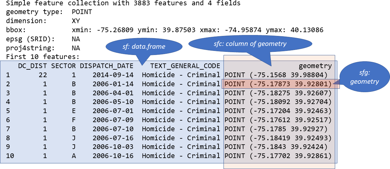
The three classes used to represent simple features are:

sf, the table (data.frame) with feature attributes and feature geometries, which contains
sfc, the list-column with the geometries for each feature (record), which is composed of
sfg, the feature geometry of an individual simple feature.

**`st_*()` functions**

Common functions to manipulate sf objects include the following:

st_read() reads a sf object,
st_write() writes a sf object,
st_crs() gets or sets a new coordinate reference system (CRS),
st_transform() transforms data to a new CRS,
st_intersection() intersects sf objects,
st_union() combines several sf objects into one,
st_simplify() simplifies a sf object,
st_coordinates() retrieves coordinates of a sf object,
st_as_sf() converts a foreign object to a sf object.

Source of some free spatial data

We can dounload some free online spatial data at
- Africa Geoportal: download
- Ethiopia Healthsites download at
- Ethiopia FEWS NET Admin Boundaries download at:
We can read a shapefile or a sf object with the st_read() function of sf.
For example, here we read the ET_Admin3_2023.shp which contains the region, zone and districts of Ethiopia.

download, read and understand Shapefiles with `sf`

Let us download data at here, Ethiopian administrative shapefile data and save from our Project folder with name Ethadmin3_2023.

Code

library(sf)
ethA3_shape <- st_read("Ethadmin3_2023/ET_Admin3_2023.shp", quiet = TRUE)

select and rename variables using dplyr package.

Code

library(dplyr)
ethR_shape <- ethA3_shape |> 
  select(FNID, ADMIN0, ADMIN1, ADMIN2, ADMIN3, Shape_Leng, 
         Shape_Area, FNID_A1, geometry) |> 
  rename(Country = ADMIN0, Region = ADMIN1, Zone = ADMIN2, Woreda = ADMIN3)

Examine

Below are a few common functions that use to examine our data. They are not from the sf package but they are very useful.

Code

# View structure and summary
head(ethR_shape, 3)

Simple feature collection with 3 features and 8 fields
Geometry type: MULTIPOLYGON
Dimension:     XY
Bounding box:  xmin: 37.51639 ymin: 13.68366 xmax: 38.56573 ymax: 14.89357
Geodetic CRS:  WGS 84
            FNID  Country Region             Zone         Woreda Shape_Leng
1 ET2023A3010101 Ethiopia Tigray Northwest Tigray Tahtay Adiyabo   3.926501
2 ET2023A3010103 Ethiopia Tigray Northwest Tigray           Zana   1.109448
3 ET2023A3010104 Ethiopia Tigray Northwest Tigray  Tahtay Koraro   2.275121
  Shape_Area    FNID_A1                       geometry
1 0.37426931 ET2023A301 MULTIPOLYGON (((37.52639 14...
2 0.04774669 ET2023A301 MULTIPOLYGON (((38.497 13.9...
3 0.06962166 ET2023A301 MULTIPOLYGON (((38.43626 14...

The sf object ethR_shape is a data.frame containing a collection with
- 1141 simple features (rows) and 9 attributes (columns) plus a list-column with the geometry of each feature.

A sf object contains the following objects of class sf, sfc and sfg:
- sf (simple feature): each row of the data.frame is a single simple feature consisting of attributes and geometry.
- sfc (simple feature geometry list-column): the geometry column of the data.frame is a list-column of class sfc with the geometry of each simple feature.
- sfg (simple feature geometry): each of the rows of the sfc list-column corresponds to the simple feature geometry (sfg) of a single simple feature.
The sf package stores geometric features in a data frame.
Geographic data is stored in the special geometry column.

Code

str(ethR_shape) # data structure

Inspect key columns and summary:

Code

# Display column names 
colnames(ethR_shape)

[1] "FNID"       "Country"    "Region"     "Zone"       "Woreda"    
[6] "Shape_Leng" "Shape_Area" "FNID_A1"    "geometry"

Subsetting Spatial Data Frames

Focus on specific regions, zones, or woredas:

Code

# Filter for a specific region (e.g., "Tigray")
tigray_data <- ethR_shape %>%
  filter(Region == "Tigray")
plot(tigray_data["Woreda"])

Code

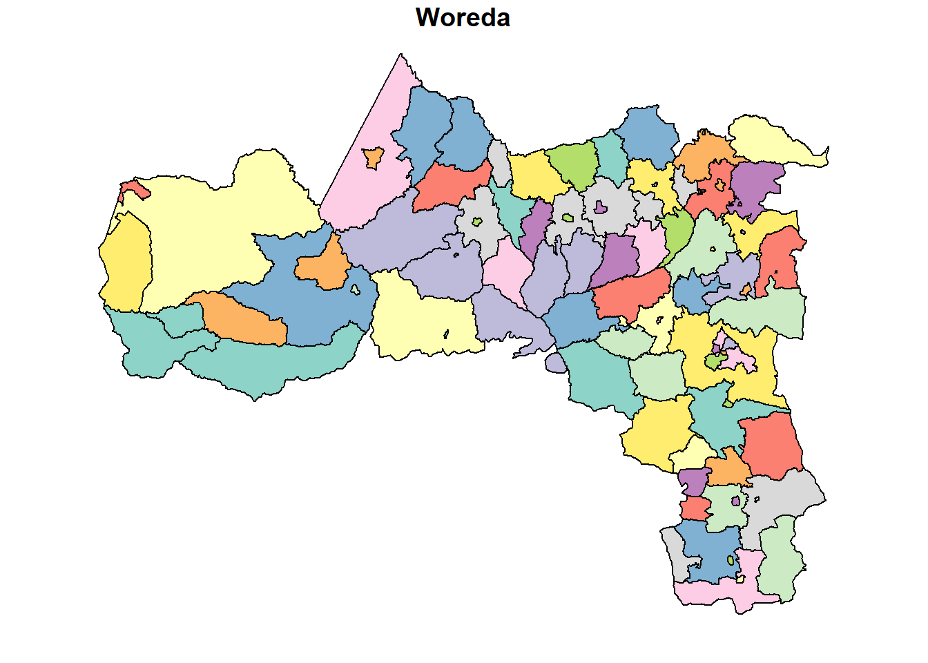
# Filter for a specific woreda (e.g., "Tahtay Adiyabo")
tahtay_adiyabo <- ethR_shape %>%
  filter(Woreda == "Tahtay Adiyabo")
plot(tahtay_adiyabo)

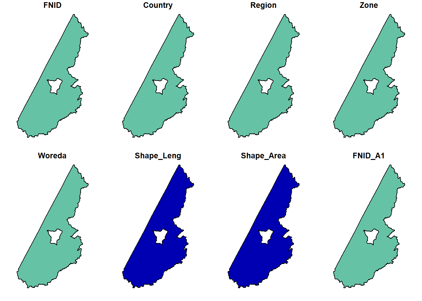
If we are interested in mapping something in the 4 regions of country: Tigray, Afar, Amhara, Oromia. The Region column in the ethR_shape.shp contains the names of each region. We will use that as our subsetting column. Let’s call it region_4.

Code

# Subset dataset to include only Four-regions.
fourR <- c("Tigray", "Afar", "Amhara", "Oromia") 
region_4 <- ethR_shape %>% 
  subset(Region %in% fourR) 

plot(region_4$geometry, col = as.factor(region_4$Region))

Spatial Transformations

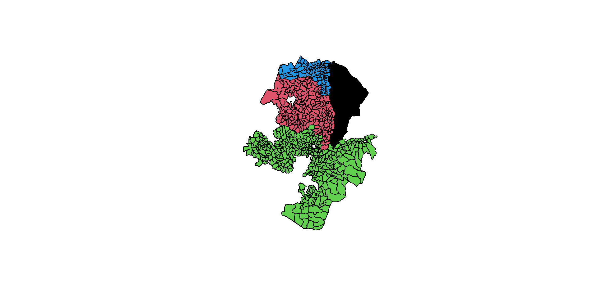
Reprojection is the transformation of geometry coordinates, from one CRS to another.
It is an important part of spatial analysis workflow, since we often need to:
- Transform several layers into the same projection, so that they can be displayed one on top of the other or so that they can be subject to a spatial operator

A vector layer can be reprojected with st_transform.

The crs can be specified in one of four ways:
- An EPSG code (e.g., 4326)
- A PROJ4 string (e.g., “+proj=longlat +datum=WGS84 +no_defs”)
- A WKT string
- A crs object of another layer, as returned by st_crs

Convert to a different coordinate reference system if needed:

Code

st_crs(ethR_shape)            # Check CRS

Coordinate Reference System:
  User input: WGS 84 
  wkt:
GEOGCRS["WGS 84",
    DATUM["World Geodetic System 1984",
        ELLIPSOID["WGS 84",6378137,298.257223563,
            LENGTHUNIT["metre",1]]],
    PRIMEM["Greenwich",0,
        ANGLEUNIT["degree",0.0174532925199433]],
    CS[ellipsoidal,2],
        AXIS["latitude",north,
            ORDER[1],
            ANGLEUNIT["degree",0.0174532925199433]],
        AXIS["longitude",east,
            ORDER[2],
            ANGLEUNIT["degree",0.0174532925199433]],
    ID["EPSG",4326]]

Code

ethR_shape <- st_transform(ethR_shape, crs = 32637)  # UTM Zone 37N
ethR_shape

Simple feature collection with 1141 features and 8 fields
Geometry type: MULTIPOLYGON
Dimension:     XY
Bounding box:  xmin: -162480.1 ymin: 376090.6 xmax: 1494221 ymax: 1646839
Projected CRS: WGS 84 / UTM zone 37N
First 10 features:
             FNID  Country Region             Zone                Woreda
1  ET2023A3010101 Ethiopia Tigray Northwest Tigray        Tahtay Adiyabo
2  ET2023A3010103 Ethiopia Tigray Northwest Tigray                  Zana
3  ET2023A3010104 Ethiopia Tigray Northwest Tigray         Tahtay Koraro
4  ET2023A3010105 Ethiopia Tigray Northwest Tigray                Asgede
5  ET2023A3010106 Ethiopia Tigray Northwest Tigray              Tselemti
6  ET2023A3010107 Ethiopia Tigray Northwest Tigray          Sheraro town
7  ET2023A3010108 Ethiopia Tigray Northwest Tigray Shire Endaslasie town
8  ET2023A3010109 Ethiopia Tigray Northwest Tigray             Selekleka
9  ET2023A3010110 Ethiopia Tigray Northwest Tigray        Seyemti Adyabo
10 ET2023A3010111 Ethiopia Tigray Northwest Tigray             Adi Daero
   Shape_Leng  Shape_Area    FNID_A1                       geometry
1   3.9265010 0.374269311 ET2023A301 MULTIPOLYGON (((340975.3 15...
2   1.1094484 0.047746694 ET2023A301 MULTIPOLYGON (((445673.4 15...
3   2.2751214 0.069621658 ET2023A301 MULTIPOLYGON (((439235.7 15...
4   2.3274188 0.134341222 ET2023A301 MULTIPOLYGON (((388463.3 15...
5   2.1683607 0.153435050 ET2023A301 MULTIPOLYGON (((381572.5 15...
6   0.4018419 0.006060853 ET2023A301 MULTIPOLYGON (((372705.9 15...
7   0.1477838 0.001221733 ET2023A301 MULTIPOLYGON (((424871 1561...
8   1.3106139 0.033449913 ET2023A301 MULTIPOLYGON (((441545.7 15...
9   1.3794723 0.061695376 ET2023A301 MULTIPOLYGON (((432113.4 16...
10  1.5071146 0.056097753 ET2023A301 MULTIPOLYGON (((428420.1 15...

Visualize the Data

If the changing of our data worked, we should be able to plot our data.. Let’s plot country.

Code

plot(ethR_shape)

So what happened?

Well, if you only use the plot() function, that particular shapefile will plot not only the shapefile geometry but also the geometry for every column in the dataset (except for the geometry column)
- which contains the spatial data
- the other columns are our tabular descriptive data).

Above are 9 maps. How many columns were there? Check code below:

Code

ncol(ethR_shape)-1

[1] 8

checking the number of columns, subtracting 1 as the geometry column doesn’t plot

st_geometry() makes our life easier.
The function goes inside the plot() function and the dataset we want to plot goes inside. Like this:

st_geometry()

Code

plot(st_geometry(ethR_shape), col = 'lightblue', border = 'darkblue')

If we want just the non-geometric part (the attributes), it can be extracted with st_drop_geometry which returns a data.frame:

Code

attrdata <- st_drop_geometry(ethR_shape)
head(attrdata)

            FNID  Country Region             Zone         Woreda Shape_Leng
1 ET2023A3010101 Ethiopia Tigray Northwest Tigray Tahtay Adiyabo  3.9265010
2 ET2023A3010103 Ethiopia Tigray Northwest Tigray           Zana  1.1094484
3 ET2023A3010104 Ethiopia Tigray Northwest Tigray  Tahtay Koraro  2.2751214
4 ET2023A3010105 Ethiopia Tigray Northwest Tigray         Asgede  2.3274188
5 ET2023A3010106 Ethiopia Tigray Northwest Tigray       Tselemti  2.1683607
6 ET2023A3010107 Ethiopia Tigray Northwest Tigray   Sheraro town  0.4018419
   Shape_Area    FNID_A1
1 0.374269311 ET2023A301
2 0.047746694 ET2023A301
3 0.069621658 ET2023A301
4 0.134341222 ET2023A301
5 0.153435050 ET2023A301
6 0.006060853 ET2023A301

Or use ggplot2

Code

library(ggplot2)
ggplot(ethR_shape) +
  geom_sf(aes(fill = Region)) +
  theme_minimal() +
  labs(title = "Regions of Ethiopia", fill = "Region")

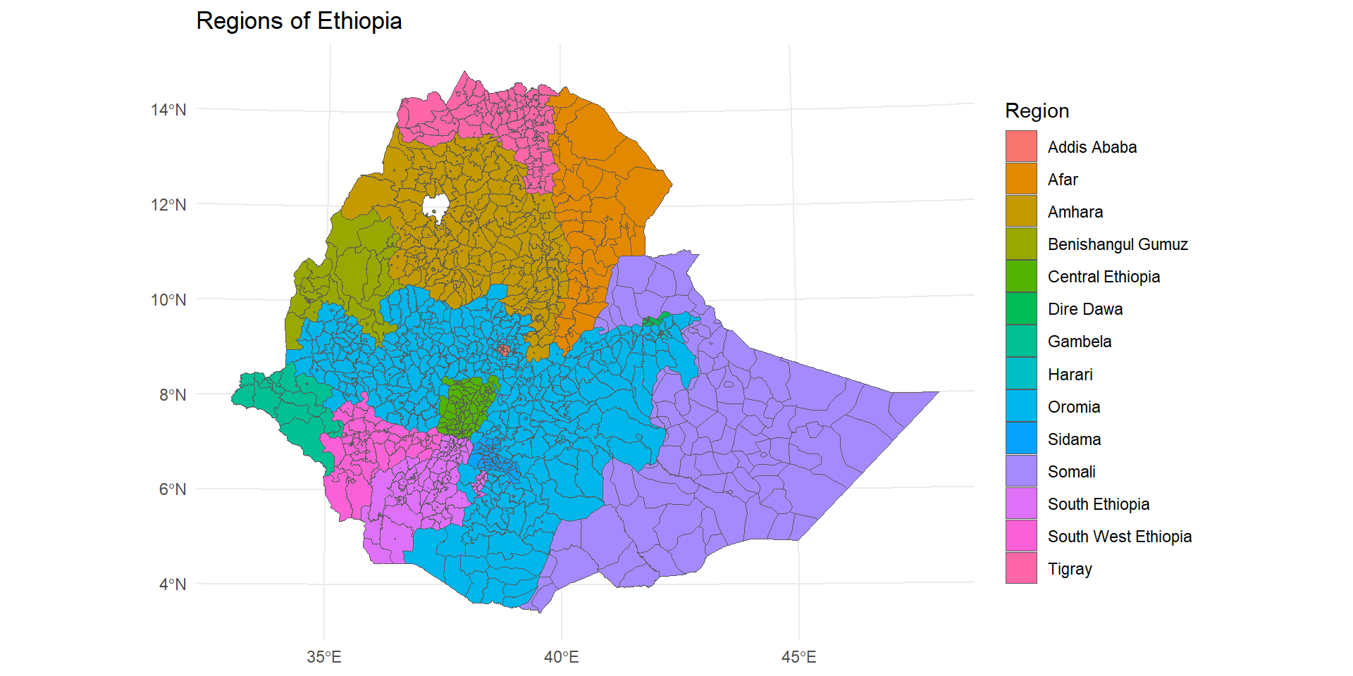
We can delete some of the polygons by taking a subset of the rows of map.

Code

map <- ethR_shape %>%
  st_filter(ethR_shape[ethR_shape$Region %in% c("Tigray", "Oromia"), ])

ggplot(map) +
  geom_sf(aes(fill = "gray")) +
  theme_minimal()

Geometric calculations

Geometric operations on vector layers can conceptually be divided into three groups according to their output:

Numericvalues —Functions that summarize geometrical properties of:
- A single layer—e.g., area, length
- A pair of layers—e.g., distance
Logicalvalues —Functions that evaluate whether a certain condition holds true, regarding:
- A single layer—e.g., geometry is valid
- A pair of layers—e.g., feature A intersects feature B
Spatial layers —Functions that create a new layer based on:
- A single layer—e.g., centroid, buffer
- A pair of layers—e.g., intersection area

Numeric

There are several functions to calculate numeric geometric properties of vector layers in package sf:

st_length—Length
st_area—Area
st_distance—Distance
st_bbox—Bounding box
st_dimension—Dimensions (0 = points, 1 = lines, 2 = polygons)
For example, we can calculate the area of each feature in the ethR_shape layer using st_area.

The result is assigned to a new attribute named area in ethR_shape:

Code

ethR_shape $area = st_area(ethR_shape )
ethR_shape$area = st_area(ethR_shape )
head(ethR_shape, 3)

Simple feature collection with 3 features and 9 fields
Geometry type: MULTIPOLYGON
Dimension:     XY
Bounding box:  xmin: 339878 ymin: 1512792 xmax: 453079 ymax: 1646839
Projected CRS: WGS 84 / UTM zone 37N
            FNID  Country Region             Zone         Woreda Shape_Leng
1 ET2023A3010101 Ethiopia Tigray Northwest Tigray Tahtay Adiyabo   3.926501
2 ET2023A3010103 Ethiopia Tigray Northwest Tigray           Zana   1.109448
3 ET2023A3010104 Ethiopia Tigray Northwest Tigray  Tahtay Koraro   2.275121
  Shape_Area    FNID_A1                       geometry             area
1 0.37426931 ET2023A301 MULTIPOLYGON (((340975.3 15... 2152127259 [m^2]
2 0.04774669 ET2023A301 MULTIPOLYGON (((445673.4 15...  570617621 [m^2]
3 0.06962166 ET2023A301 MULTIPOLYGON (((439235.7 15...  830999755 [m^2]

The resulting area values, just like any other numeric calculations in sf, are returned as object of class units:

Code

class(ethR_shape$area)

[1] "units"

A units object is basically a numeric vector associated with units of measurement. We can transform units measurements to different units, with function set_units from package units.
First, we load the units library:
Then, we make the transformation to \(km°2\) units:

Code

library(units)
ethR_shape$area = set_units(ethR_shape$area, "km^2")

Code

plot(ethR_shape["area"])

Spatial

sf provides common geometry-generating functions applicable to individual geometries, such as:

st_centroid—Centroids
st_buffer—Buffer
st_sample—Random sample points
st_convex_hull—Convex hull
st_voronoi—Voronoi polygons

For example, to calculate the centroids of the “wored” polygons we can use the st_centroid function as follows:

Code

ethR_shape <- st_make_valid(ethR_shape)
ethR_shape_ctr = st_centroid(ethR_shape)

They can be plotted as follows

Code

plot(st_geometry(ethR_shape), border = "grey") 
plot(st_geometry(ethR_shape_ctr), col = "blue", pch = 3, add = TRUE)

`stars`: Rasters

Geometric operations on rasters can be done with package stars:

Accessing cell values—As matrix / array, Extracting to points / lines / polygons
Raster algebra—Arithmetic (+, -, …), Math (sqrt, log10, …), logical (!, ==, >, …), summary (mean, max, …), Masking
Changing resolution and extent—Cropping, Mosaic, Resampling, Reprojection
Transformations—Raster <-> Points / Contour lines / Polygons

Overview of spatial and non-spatial data analysis framework

Coming soon!

Spatial Exploratory Data Analysis

Coming soon!

Investigating spatial dependence

Coming soon!

Spatial modeling framework

Coming soon!

Geostatistical Modeling

Coming soon!

Outlines ….. (1)

Outlines ….. (2)

Source, Format, and Types of Spatial Data

What is GIS? What is spatial data and why should we use it?

Spatial Data Formats

Spatial Data Formats Categorized by Type

Spatial Data Types

Vector Data: Overview

Raster Data: Overview

What are the most common Vector data formats?

What are the most common Raster data formats?

What are the components of spatial data

Coordinate Reference Systems (CRS):

Commonly Used EPSG Codes

CRS Formats

Basic R Packages for Spatial Data Analysis

Basic R Packages for Spatial Data Analysis

Install required Packages

sf() package

st_*() functions

Source of some free spatial data

download, read and understand Shapefiles with sf

Examine

Inspect key columns and summary:

Subsetting Spatial Data Frames

Spatial Transformations

Visualize the Data

st_geometry()

Geometric calculations

Numeric

Spatial

stars: Rasters

Overview of spatial and non-spatial data analysis framework

Spatial Exploratory Data Analysis

Investigating spatial dependence

Spatial modeling framework

Geostatistical Modeling

`sf()` package

**`st_*()` functions**

download, read and understand Shapefiles with `sf`

`stars`: Rasters