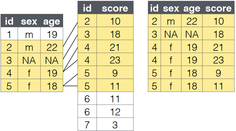
Merging data

National Data Management Center for Health (NDMC) at EPHI

Data mergining

Why Merging Matters in Public Health

• Combine demographic & clinical data
• Link longitudinal health records
• Merge survey responses with medical data
• Integrate multiple data sources for cohort studies

• The 4 mutating join verbs:
• left_join()
• right_join()
• inner_join()
• full_join()

• The 2 binding join verbs:

• bind_rows()

• bind_cols()

• The 2 filtering join verbs:
• semi_join()
• anti_join()

• The 3 set operations:
• intersect()
• union()
• setdiff()

• All the joins have this basic syntax: *_join(x, y, by = NULL, suffix = c(".x", ".y")

• x = the first (left) table

• y = the second (right) table

• by = what columns to match on. If you leave this blank, it will match on all columns with the same names in the two tables.

• suffix = if columns have the same name in the two tables, but you aren’t joining by them, they get a suffix to make them unambiguous.

• This defaults to “.x” and “.y”, but you can change it to something more meaningful.

Sample Health Datasets

1. Patient Demographics (Synthetic)

library(tibble)
clinic_data <- tibble(
  patient_id = c("P001", "P002", "P003", "P004"),
  age = c(35, 28, 42, 31),
  bmi = c(22.1, 26.5, 29.8, 24.3),
  smoking_status = c("former", "never", "current", "never")
)

2. Clinical Measurements

lab_data <- tibble(
  patient_id = c("P002", "P003", "P003", "P005"),
  visit_date = as.Date(c("2023-01-15", "2023-02-01", 
                         "2023-03-01", "2023-01-20")),
  sbp = c(120, 135, 140, 128),
  dbp = c(80, 85, 90, 82))

left_join(): Preserve Clinic Records

What it does:

• Retains all rows from the left (first) table

• Adds matching columns from the right (second) table

• Fills NA where no match exists

• left_joint()

library(dplyr)
left_join(clinic_data, lab_data, by = "patient_id") %>% 
  arrange(patient_id) %>% head(4) 

# A tibble: 4 × 7
  patient_id   age   bmi smoking_status visit_date   sbp   dbp
  <chr>      <dbl> <dbl> <chr>          <date>     <dbl> <dbl>
1 P001          35  22.1 former         NA            NA    NA
2 P002          28  26.5 never          2023-01-15   120    80
3 P003          42  29.8 current        2023-02-01   135    85
4 P003          42  29.8 current        2023-03-01   140    90

• Merging patient registries with lab results

• Preserving all patients from primary clinic records

• The order of the clinic_data and lab_data tables is different.

left_join(lab_data, clinic_data, by = "patient_id") %>% 
  arrange(patient_id) %>% head(4)  

# A tibble: 4 × 7
  patient_id visit_date   sbp   dbp   age   bmi smoking_status
  <chr>      <date>     <dbl> <dbl> <dbl> <dbl> <chr>         
1 P002       2023-01-15   120    80    28  26.5 never         
2 P003       2023-02-01   135    85    42  29.8 current       
3 P003       2023-03-01   140    90    42  29.8 current       
4 P005       2023-01-20   128    82    NA  NA   <NA>          

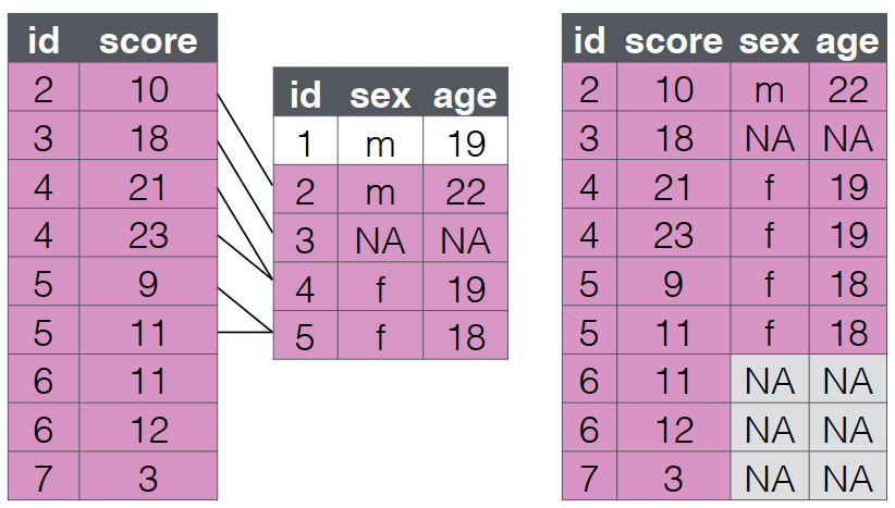
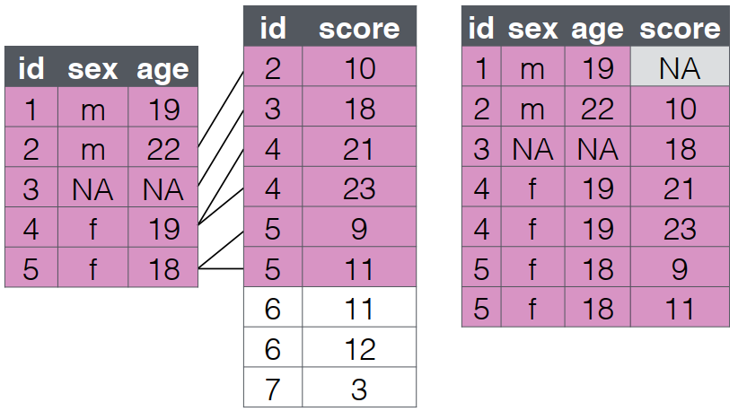
right_join()

• A right_join keeps all the data from the second (right) table and joins anything that matches from the first (left) table.

inner_join(): Complete Cases Only

What it does:

• Returns only rows with matches in both tables
• Filters out non-matching records
• An inner_join returns all the rows that have a match in the other table.

inner_join(clinic_data, lab_data, by = "patient_id") %>% 
  knitr::kable()

patient_id	age	bmi	smoking_status	visit_date	sbp	dbp
P002	28	26.5	never	2023-01-15	120	80
P003	42	29.8	current	2023-02-01	135	85
P003	42	29.8	current	2023-03-01	140	90

• Creating analysis datasets with complete information
• Identifying patients with both survey and clinical data

full_join()

What it does:

• A full_join lets you join up rows in two tables while keeping all of the information from both tables.
• If a row doesn’t have a match in the other table, the other table’s column values are set to NA.

full_join(clinic_data, lab_data, by = "patient_id")

# A tibble: 6 × 7
  patient_id   age   bmi smoking_status visit_date   sbp   dbp
  <chr>      <dbl> <dbl> <chr>          <date>     <dbl> <dbl>
1 P001          35  22.1 former         NA            NA    NA
2 P002          28  26.5 never          2023-01-15   120    80
3 P003          42  29.8 current        2023-02-01   135    85
4 P003          42  29.8 current        2023-03-01   140    90
5 P004          31  24.3 never          NA            NA    NA
6 P005          NA  NA   <NA>           2023-01-20   128    82

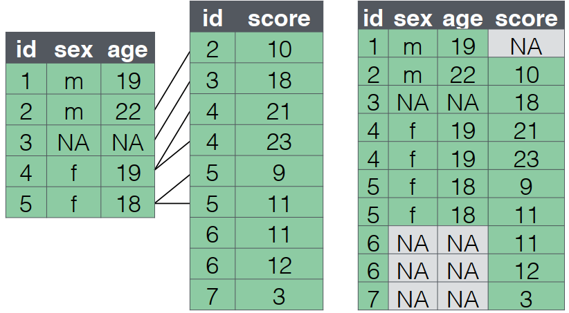
semi_join()

• A semi_join filters left table to rows with matches in right table
• Keeps only left table columns

semi_join(clinic_data, lab_data, by = "patient_id")

# A tibble: 2 × 4
  patient_id   age   bmi smoking_status
  <chr>      <dbl> <dbl> <chr>         
1 P002          28  26.5 never         
2 P003          42  29.8 current       

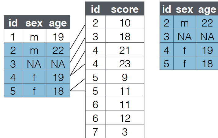
• Here in this data case: Find patients with lab results

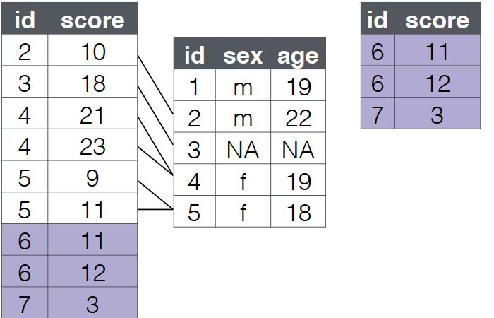
anti_join(): Identify Missing Data

• A anti_join() return all rows from the left table where there are not matching values in the right table, keeping just columns from the left table.

• anti_join().

anti_join(clinic_data, lab_data, by = "patient_id") %>% 
  knitr::kable()

patient_id	age	bmi	smoking_status
P001	35	22.1	former
P004	31	24.3	never

• In this data case: Identify patients needing follow-up ::: {style=“text-align:center”}

• Order matters in an anti_join().

anti_join(lab_data,clinic_data, by = "patient_id") %>% 
  knitr::kable()

patient_id	visit_date	sbp	dbp
P005	2023-01-20	128	82

:::::::

Find patients needing follow-up lab tests

Real-world Example: Birth Weight Analysis Birth Weight Data (MASS::birthwt)

birthwt_modified <- MASS::birthwt %>%
  mutate(
    patient_id = paste0("M", 1:n()),
    low = factor(low, labels = c("Normal", "Low")),
    smoke = factor(smoke, labels = c("Non-smoker", "Smoker"))) %>%   
  select(patient_id, low, age = age, weight = lwt, smoke)

Postnatal Follow-up Data (Synthetic)

followup_data <- tibble(
  patient_id = c("M12", "M15", "M42", "M88"),
  infant_weight_6mo = c(7.2, 6.8, 7.5, 6.9),
  breastfeeding_duration = c(6, 5, NA, 4))

1. full_join(): Comprehensive Birth Cohort

• Combine prenatal and postnatal data for longitudinal analysis

right_join(birthwt_modified, followup_data, by = "patient_id") %>% 
  select(patient_id, low, smoke, infant_weight_6mo)  %>% 
  knitr::kable()

patient_id	low	smoke	infant_weight_6mo
M12	Normal	Non-smoker	7.2
M15	Normal	Smoker	6.8
M42	Normal	Non-smoker	7.5
M88	Normal	Non-smoker	6.9

2. semi_join(): Smoking Mothers with Follow-up

• Identify smoking mothers in follow-up program

birthwt_modified %>% 
  semi_join(followup_data, by = "patient_id") %>% 
  filter(smoke == "Smoker") %>% 
  knitr::kable()

	patient_id	low	age	weight	smoke
100	M15	Normal	18	100	Smoker

bind_rows()

• You can combine the rows of two tables with bind_rows.
• Here we’ll add subject data for subjects 6-9 and bind that to the original subject table.

new_patients <- tibble(
  patient_id = c("P4", "P5"),
  age = c(55, 38),
  smoking_status = c("Never", "Current")
)

bind_rows(clinic_data, new_patients)

# A tibble: 6 × 4
  patient_id   age   bmi smoking_status
  <chr>      <dbl> <dbl> <chr>         
1 P001          35  22.1 former        
2 P002          28  26.5 never         
3 P003          42  29.8 current       
4 P004          31  24.3 never         
5 P4            55  NA   Never         
6 P5            38  NA   Current       

bind_rows(subject, new_subjects)

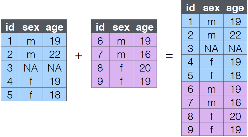
• The columns just have to have the same names, they don’t have to be in the same order.

• Any columns that differ between the two tables will just have NA values for entries from the other table.

• If a row is duplicated between the two tables (like id 5 below), the row will also be duplicated in the resulting table.